Page 60 - Circuit Analysis II with MATLAB Applications

Chapter 1 Second Order Circuits

By substitution into (1) we find the total solution as

v t = v + v Cn = 100 36e – 2t + 16e – 3t
–
Cf
C
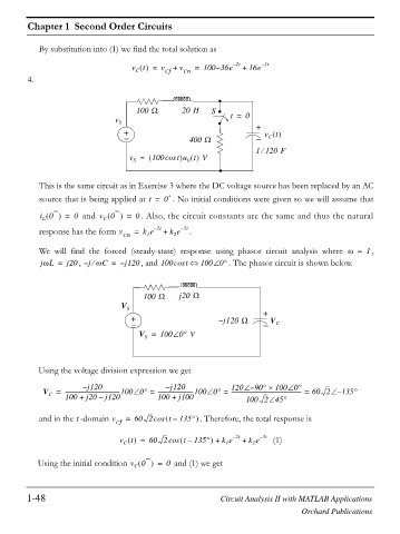
4.
`
100 : 20 H S
v S t = 0

+ + v t
400 : C
1120 F
e
t
v = 100cos u t V

S
0
This is the same circuit as in Exercise 3 where the DC voltage source has been replaced by an AC
source that is being applied at t = 0 + . No initial conditions were given so we will assume that

i 0 L = 0 and v 0 C = 0 . Also, the circuit constants are the same and thus the natural
response has the form v Cn = k e – 2t + k e – 3t .
1
2
We will find the forced (steady-state) response using phasor circuit analysis where Z = , 1
jZL = j20 , j– ZCe = – j120 , and 100cos t œ 100 0q . The phasor circuit is shown below.
‘

`
100 : j20 :
V S
+ j – 120 : + V
C
V = 100 0q V
‘
S

Using the voltage division expression we get
– j120 – j120 120 – 90q u 100 0q
‘
‘
V = ----------------------------------------100 0q‘ = --------------------------100 0q‘ = ---------------------------------------------------- = 60 2 – 135q
‘
C
100 +
j120
100 +
j100
j20 –
‘
100 2 45q
and in the -domain v Cf = 60 2cos t – 135q . Therefore, the total response is
t
v t = 60 2cos t – 135q + k e – 2t + k e – 3t (1)

C
1
2

Using the initial condition v 0 C = 0 and (1) we get
1-48 Circuit Analysis II with MATLAB Applications
Orchard Publications