Page 58 - Circuit Analysis II with MATLAB Applications

Chapter 1 Second Order Circuits

t v C (t) i L (t)
v C (t)
0.000 -0.014 -0.002
0.010 0.0313 0.198
0.020 0.1677 0.395
150
0.030 0.394 0.591
0.040 0.7094 0.784 50
0.050 1.1129 0.975
0.060 1.6034 1.164 -50 0 3 6 9 12
0.070 2.1798 1.35
0.080 2.8407 1.534
i L (t)
0.090 3.5851 1.714
0.100 4.4115 1.892
0.110 5.3185 2.066 10
0.120 6.3046 2.238
0.130 7.3684 2.405
0.140 8.5082 2.57 0 3 6 9 12
0.150 9.7224 2.73 -10
0.160 11.009 2.887
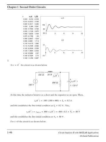
3.

At t = 0 the circuit is as shown below.

`
100 : 20 H
i 0
L
+
+ v 0
400 : C
100 V 1 120 F
e

At this time the inductor behaves as a short and the capacitor as an open. Then,

i 0 L 100 = 100 + 400 = I = 0.2 A
e
0
and this establishes the first initial condition as I = 0.2 A . Also,
0

v 0 C = v 400 : = 400 u i 0 = 400 u 0.2 = V = 80 V
L
0
and this establishes the first initial condition as V = 80 V .
0
For t ! 0 the circuit is as shown below.

1-46 Circuit Analysis II with MATLAB Applications
Orchard Publications