Page 266 - Classification Parameter Estimation & State Estimation An Engg Approach Using MATLAB
P. 266
STATE ESTIMATION IN PRACTICE 255
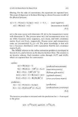
filtering. For the sake of convenience, the equations are repeated here.
The point of departure in Kalman filtering is a linear-Gaussian model of
the physical process:
xði þ 1Þ¼ FðiÞxðiÞþ LðiÞuðiÞþ wðiÞ i ¼ 0;1;... ðstate equationÞ
zðiÞ¼ HðiÞxðiÞþ vðiÞ ðmeasurement modelÞ
ð8:1Þ
x(i) is the state vector with dimension M. z(i) is the measurement vector
with dimension N. The process noise w(i) and measurement noise v(i)
are white Gaussian noise sequences, zero mean, and with covariance
matrix C w (i) and C v (i), respectively. Process noise and measurement
noise are uncorrelated: C wv (i) ¼ 0. The prior knowledge is that x(0)
has a Gaussian distribution with expectation E[x(0)] and covariance
matrix C x (0).
The MMSE solution to the online estimation problem is developed in
Section 4.2.1, and is known as the discrete Kalman filter. The solution is
an iterative scheme. Each iteration cycles through (4.27) and (4.28),
which are repeated here for convenience:
update :
z
^ zðiÞ¼ HðiÞxðiji 1Þ
ðpredicted measurementÞ
T
SðiÞ¼ HðiÞCðiji 1ÞH ðiÞþC v ðiÞ
ðinnovation matrixÞ
T 1
KðiÞ¼ Cðiji 1ÞH ðiÞS ðiÞ ðKalman gain matrixÞ
z
ð
xðijiÞ¼ xðiji 1ÞþKðiÞ zðiÞ ^ zðiÞÞ
ðupdated estimateÞ
T
CðijiÞ¼ Cðiji 1Þ KðiÞSðiÞK ðiÞ ðerror covariance matrixÞ
prediction :
x
xðiþ1jiÞ¼ FðiÞ xðijiÞþLðiÞuðiÞ ðpredictionÞ
T ðpredicted state covarianceÞ
Cðiþ1jiÞ¼ FðiÞCðijiÞF ðiÞþC w ðiÞ
ð8:2Þ
The iterative procedure is initiated with the prediction for i ¼ 0 set equal
to the prior:
def def
xð0j 1Þ¼E½xð0Þ and Cð0j 1Þ¼C x ð0Þ:

