Page 268 - Classification Parameter Estimation & State Estimation An Engg Approach Using MATLAB

SYSTEM IDENTIFICATION 257

1
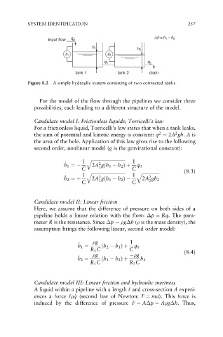
input flow q 0 ∆h = h – h 2
h 1 h 2
z 1 z 2
q 1 q 2

tank 1 tank 2 drain

Figure 8.2 A simple hydraulic system consisting of two connected tanks

For the model of the flow through the pipelines we consider three
possibilities, each leading to a different structure of the model.

Candidate model I: Frictionless liquids; Torricelli’s law
For a frictionless liquid, Torricelli’s law states that when a tank leaks,
2
2
the sum of potential and kinetic energy is constant: q ¼ 2A gh. A is
the area of the hole. Application of this law gives rise to the following
second order, nonlinear model (g is the gravitational constant):

_ 1 q ffiffiffiffiffiffiffiffiffiffiffiffiffiffiffiffiffiffiffiffiffiffiffiffiffiffiffiffiffiffi 1
2
h h 1 ¼ 2A gðh 1 h 2 Þ þ q 0
1
C C
ð8:3Þ
q
ffiffiffiffiffiffiffiffiffiffiffiffiffiffiffiffiffiffiffiffiffiffiffiffiffiffiffiffiffiffi
q
ffiffiffiffiffiffiffiffiffiffiffiffiffiffiffiffi
_ 1 2 1 2
h h 2 ¼þ 2A gðh 1 h 2 Þ 2A gh 2
1
2
C C
Candidate model II: Linear friction
Here, we assume that the difference of pressure on both sides of a
pipeline holds a linear relation with the flow: p ¼ Rq. The para-
meter R is the resistance. Since p ¼ g h ( is the mass density), the
assumption brings the following linear, second order model:
_ g 1
h h 1 ¼ ðh 2 h 1 Þþ q 0
R 1 C C ð8:4Þ
_ g g
h h 2 ¼ ðh 1 h 2 Þþ h 2
R 1 C R 2 C

Candidate model III: Linear friction and hydraulic inertness
A liquid within a pipeline with a length ‘ and cross-section A experi-
ences a force ‘ _ q (second law of Newton: F ¼ ma). This force is
q
induced by the difference of pressure F ¼ A p ¼ A g h. Thus,