Page 269 - Classification Parameter Estimation & State Estimation An Engg Approach Using MATLAB

258 STATE ESTIMATION IN PRACTICE

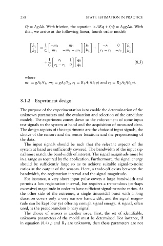
‘_ q ¼ Ag h. With friction, the equation is ARq þ ‘ _ q ¼ A g h. With
q
q
that, we arrive at the following linear, fourth order model:

€ 0 _

h h 1 1 m 1 m 1 h 1 r 1 h h 1
€ ¼ þ _
h h 2 C m 1 m 1 m 2 h 2 r 1 r 2 r 2 h h 2
1 r 1 1 q 0
þ ð8:5Þ
C r 2 r 1 0 _ q q 0

where
m 1 ¼ gA 1 /‘ 1 , m 2 ¼ gA 2 /‘ 2 , r 1 ¼ R 1 A 1 /(‘ 1 ) and r 2 ¼ R 2 A 2 /(‘ 2 ).

8.1.2 Experiment design

The purpose of the experimentation is to enable the determination of the
unknown parameters and the evaluation and selection of the candidate
models. The experiment comes down to the enforcement of some input
test signals to the system at hand and the acquisition of measured data.
The design aspects of the experiments are the choice of input signals, the
choice of the sensors and the sensor locations and the preprocessing of
the data.
The input signals should be such that the relevant aspects of the
system at hand are sufficiently covered. The bandwidth of the input sig-
nal must match the bandwidth of interest. The signal magnitude must be
in a range as required by the application. Furthermore, the signal energy
should be sufficiently large so as to achieve suitable signal-to-noise
ratios at the output of the sensors. Here, a trade-off exists between the
bandwidth, the registration interval and the signal magnitude.
For instance, a very short input pulse covers a large bandwidth and
permits a low registration interval, but requires a tremendous (perhaps
excessive) magnitude in order to have sufficient signal-to-noise ratios. At
the other side of the extremes, a single sinusoidal burst with a long
duration covers only a very narrow bandwidth, and the signal magni-
tude can be kept low yet offering enough signal energy. A signal, often
used, is the pseudorandom binary signal.
The choice of sensors is another issue. First, the set of identifiable,
unknown parameters of the model must be determined. For instance, if
in equation (8.4) and R 1 are unknown, then these parameters are not