Page 271 - Classification Parameter Estimation & State Estimation An Engg Approach Using MATLAB

260 STATE ESTIMATION IN PRACTICE

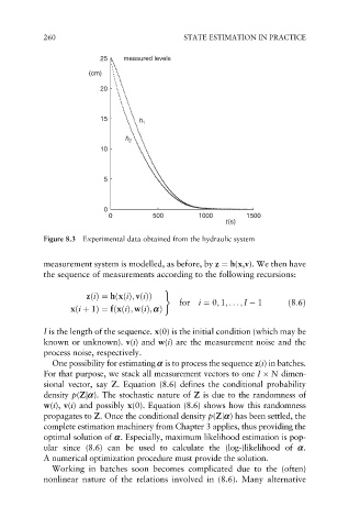
25 measured levels
(cm)
20

15 h 1

h 2
10

5

0
0 500 1000 1500
t(s)
Figure 8.3 Experimental data obtained from the hydraulic system

measurement system is modelled, as before, by z ¼ h(x,v). We then have
the sequence of measurements according to the following recursions:

)
zðiÞ¼ hxðiÞ; vðiÞÞ
ð
for i ¼ 0; 1; .. . ; I 1 ð8:6Þ
xði þ 1Þ¼ fxðiÞ; wðiÞ; aÞ
ð
I is the length of the sequence. x(0) is the initial condition (which may be
known or unknown). v(i) and w(i) are the measurement noise and the
process noise, respectively.
One possibility for estimating a is to process the sequence z(i) in batches.
For that purpose, we stack all measurement vectors to one I N dimen-
sional vector, say Z. Equation (8.6) defines the conditional probability
density p(Zja). The stochastic nature of Z is due to the randomness of
w(i), v(i) and possibly x(0). Equation (8.6) shows how this randomness
propagates to Z. Once the conditional density p(Zja) has been settled, the
complete estimation machinery from Chapter 3 applies, thus providing the
optimal solution of a. Especially, maximum likelihood estimation is pop-
ular since (8.6) can be used to calculate the (log-)likelihood of a.
A numerical optimization procedure must provide the solution.
Working in batches soon becomes complicated due to the (often)
nonlinear nature of the relations involved in (8.6). Many alternative