Page 276 - Classification Parameter Estimation & State Estimation An Engg Approach Using MATLAB

SYSTEM IDENTIFICATION 265

The parameters n are found by estimating the correlation coefficients r k
and solving (8.11).
2
The parameter is obtained by multiplying (8.9) by x(i) and taking
w
expectations:
M
2 X 2 2
¼ a n r k þ w ð8:12Þ
x
x
n¼1
2
2
Estimation of and solving (8.12) gives us the estimate of .
x
w
The order of the system can be retrieved by a concept called the
partial autocorrelation function. Suppose that an AR sequence x(i)has
been observed with unknown order M. The procedure for the identifi-
cation of this sequence is to first estimate the correlation coefficients r k
r
yielding estimates ^ r k . Then, for a number of hypothesized orders
^
^
M M ¼ 1, 2, 3, .. . we estimate the AR coefficients ^ k, ^ M for k ¼ 1, .. . , M
M

M
^
(the subscript M has been added to discriminate between coefficients of
M
different orders). From these coefficients, the last one of each sequence,
, is called the partial autocorrelation function. It can be
i.e. ^ ^ M, ^ M
M
M
proven that:
^
¼ 0 for M M > M ð8:13Þ
^ M; ^ M
M
M
drops down to
M M
Thus, the order M is determined by checking where ^ ^ M, ^ M
near zero.
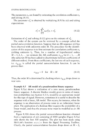
Example 8.5 AR model of a pseudorandom binary sequence
Figure 8.5(a) shows a realization of a zero mean, pseudorandom
binary sequence. A discrete Markov model, given in terms of transi-
tion probabilities (see Section 4.3.1), would be an appropriate model
for this type of signal. However, sometimes it is useful to describe the
sequence with a linear, AR model. This occurs, for instance, when the
sequence is an observation of process noise in an (otherwise) linear
plant. The application of a Kalman filter requires the availability of a
linear model, and thus the process noise must be modelled as an AR
process.
Figure 8.5(b) shows the partial autocorrelation function obtained
from a registration of x(i) consisting of 4000 samples (Figure 8.5(a)
only shows the first 500 samples). The plot has been made using
MATLAB’s function aryule from the Signal Processing Toolbox.
^
Clearly, the partial autocorrelation function drops down at M ¼ 2,
M