Page 280 - Classification Parameter Estimation & State Estimation An Engg Approach Using MATLAB

OBSERVABILITY, CONTROLLABILITY AND STABILITY 269

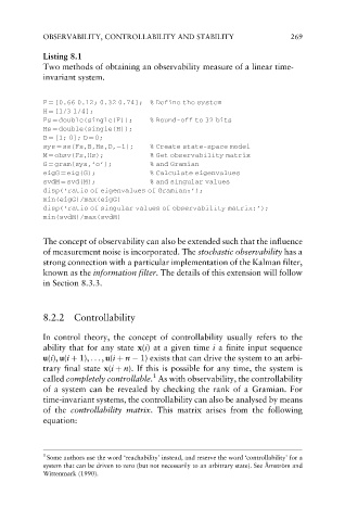
Listing 8.1
Two methods of obtaining an observability measure of a linear time-
invariant system.

F ¼ [0.66 0.12; 0.32 0.74]; % Define the system
H ¼ [1/3 1/4];
Fs ¼ double(single(F)); % Round-off to 32 bits
Hs ¼ double(single(H));
B ¼ [1; 0]; D ¼ 0;
sys ¼ ss(Fs,B,Hs,D, 1); % Create state-space model
M ¼ obsv(Fs,Hs); % Get observability matrix
G ¼ gram(sys,’o’); % and Gramian
eigG ¼ eig(G); % Calculate eigenvalues
svdM ¼ svd(M); % and singular values
disp(‘ratio of eigenvalues of Gramian:’);
min(eigG)/max(eigG)
disp(‘ratio of singular values of observability matrix:’);
min(svdM)/max(svdM)

The concept of observability can also be extended such that the influence
of measurement noise is incorporated. The stochastic observability has a
strong connection with a particular implementation of the Kalman filter,
known as the information filter. The details of this extension will follow
in Section 8.3.3.

8.2.2 Controllability

In control theory, the concept of controllability usually refers to the
ability that for any state x(i) at a given time i a finite input sequence
u(i), u(i þ 1), .. . , u(i þ n 1) exists that can drive the system to an arbi-
trary final state x(i þ n). If this is possible for any time, the system is
1
called completely controllable. As with observability, the controllability
of a system can be revealed by checking the rank of a Gramian. For
time-invariant systems, the controllability can also be analysed by means
of the controllability matrix. This matrix arises from the following
equation:

1
Some authors use the word ‘reachability’ instead, and reserve the word ‘controllability’ for a
¨
system that can be driven to zero (but not necessarily to an arbitrary state). See A ˚ mstrom and
Wittenmark (1990).