Page 284 - Classification Parameter Estimation & State Estimation An Engg Approach Using MATLAB

OBSERVABILITY, CONTROLLABILITY AND STABILITY 273

A steady state solution of the Ricatti equation gives rise to a constant
Kalman gain. The corresponding Kalman filter, derived from (8.2) and (8.21):

xði þ 1ji þ 1Þ¼ I KHÞF xðijiÞþ I KHÞLuðiÞþ Kzði þ 1Þð8:25Þ
ð
ð
with:
1
T

KðiÞ¼ PH T HPH þ C v
becomes time invariant.

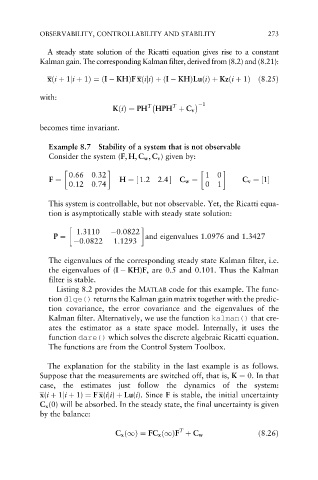
Example 8.7 Stability of a system that is not observable
Consider the system (F, H, C w , C v ) given by:

0:66 0:32 10
½
F ¼ H ¼ 1:22:4 Š C w ¼ C v ¼½1Š
0:12 0:74 01
This system is controllable, but not observable. Yet, the Ricatti equa-
tion is asymptotically stable with steady state solution:

1:3110 0:0822
P ¼ and eigenvalues 1.0976 and 1.3427
0:0822 1:1293
The eigenvalues of the corresponding steady state Kalman filter, i.e.
the eigenvalues of (I KH)F, are 0.5 and 0.101. Thus the Kalman
filter is stable.
Listing 8.2 provides the MATLAB code for this example. The func-
tion dlqe() returns the Kalman gain matrix together with the predic-
tion covariance, the error covariance and the eigenvalues of the
Kalman filter. Alternatively, we use the function kalman() that cre-
ates the estimator as a state space model. Internally, it uses the
function dare() which solves the discrete algebraic Ricatti equation.
The functions are from the Control System Toolbox.

The explanation for the stability in the last example is as follows.
Suppose that the measurements are switched off, that is, K ¼ 0. In that
case, the estimates just follow the dynamics of the system:
x(i þ 1ji þ 1) ¼ F x(iji) þ Lu(i). Since F is stable, the initial uncertainty
C x (0) will be absorbed. In the steady state, the final uncertainty is given
by the balance:

T
C x ð1Þ ¼ FC x ð1ÞF þ C w ð8:26Þ