Page 289 - Classification Parameter Estimation & State Estimation An Engg Approach Using MATLAB

278 STATE ESTIMATION IN PRACTICE

As an example, consider the following Ricatti loop:

T
SðiÞ¼ HCðiji 1ÞH þ C v
T 1
KðiÞ¼ðHCðiji 1ÞÞ S ðiÞ
ð8:30Þ
CðijiÞ¼ Cðiji 1Þ KðiÞHCðiji 1Þ
T
Cði þ 1jiÞ¼ FCðijiÞF þ C w
This loop is mathematically equivalent to (8.2), but is computationally
less expensive because the factor HC(iji 1) appears at several places
and can be reused. However, the form is prone to round-off errors:

. The part K(i)H can easily introduce asymmetries in C(iji).
. The subtraction I K(i)H can introduce negative eigenvalues.

The implementation should be used cautiously. The preferred implemen-
tation is (8.2):

T
CðijiÞ¼ Cðiji 1Þ KðiÞSðiÞK ðiÞ ð8:31Þ
It requires more operations than expression (8.30), but it is more
balanced. Therefore, the risk of introducing asymmetries is much lower.
Still, this implementation does not guarantee non-negative eigenvalues.
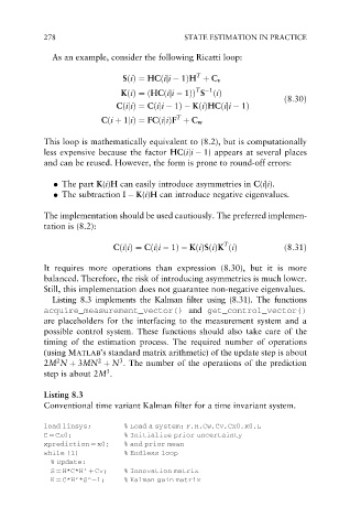
Listing 8.3 implements the Kalman filter using (8.31). The functions
acquire_measurement_vector() and get_control_vector()
are placeholders for the interfacing to the measurement system and a
possible control system. These functions should also take care of the
timing of the estimation process. The required number of operations
(using MATLAB’s standard matrix arithmetic) of the update step is about
2
2
3
2M N þ 3MN þ N . The number of the operations of the prediction
3
step is about 2M .
Listing 8.3
Conventional time variant Kalman filter for a time invariant system.

load linsys; % Load a system: F,H,Cw,Cv,Cx0,x0,L
C ¼ Cx0; % Initialize prior uncertainty
xprediction ¼ x0; % and prior mean
while (1) % Endless loop
% Update:
S ¼ H*C*H’ þ Cv; % Innovation matrix
K ¼ C*H’*S^ 1; % Kalman gain matrix