Page 290 - Classification Parameter Estimation & State Estimation An Engg Approach Using MATLAB

COMPUTATIONAL ISSUES 279

z ¼ acquire_measurement_vector();
innovation ¼ z - H*xprediction;
xestimation ¼ xprediction þ K*innovation;
C ¼ C - K*S*K’;
% Prediction:
u ¼ get_control_vector();
xprediction ¼ F*xestimation þ L*u;
C ¼ F*C*F’ þ Cw;
end

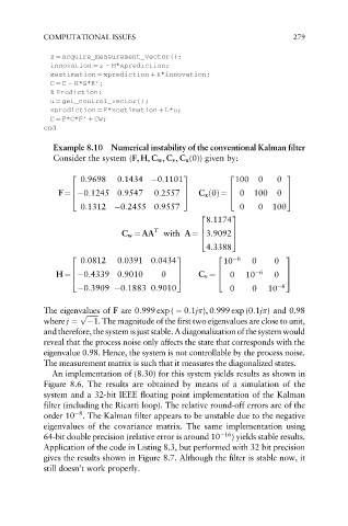
Example 8.10 Numerical instability of the conventional Kalman filter
Consider the system (F, H, C w , C v , C x (0)) given by:

0:9698 0:1434 0:1101 100 0 0
2 3 2 3
F ¼ 0:1245 0:9547 7 6 0 100 7
6
4 0:2557 5 C x ð0Þ¼ 4 0 5
0:1312 0:2455 0:9557 0 0 100
8:1174
2 3
C w ¼ AA T 6 7
4
with A¼ 3:90925
4:3388
0:0812 0:0391 0:0434 10 0 0
2 3 2 6 3
H ¼ 0:4339 0:9010 0 7 6 0 10 6 7
6
4 5 C v ¼ 4 0 5
0:3909 0:1883 0:9010 0 0 10 6
The eigenvalues of F are 0:999 exp ( 0:1j ), 0:999 exp (0:1j ) and 0.98
p ffiffiffiffiffiffiffi
where j ¼ 1. The magnitude of the first two eigenvalues are close to unit,
andtherefore, the systemis just stable. Adiagonalizationofthesystem would
reveal that the process noise only affects the state that corresponds with the
eigenvalue 0.98. Hence, the system is not controllable by the process noise.
The measurement matrix is such that it measures the diagonalized states.
An implementation of (8.30) for this system yields results as shown in
Figure 8.6. The results are obtained by means of a simulation of the
system and a 32-bit IEEE floating point implementation of the Kalman
filter (including the Ricatti loop). The relative round-off errors are of the
8
order 10 . The Kalman filter appears to be unstable due to the negative
eigenvalues of the covariance matrix. The same implementation using
64-bit double precision (relative error is around 10 16 ) yields stable results.
Application of the code in Listing 8.3, but performed with 32 bit precision
gives the results shown in Figure 8.7. Although the filter is stable now, it
still doesn’t work properly.