Page 293 - Classification Parameter Estimation & State Estimation An Engg Approach Using MATLAB

282 STATE ESTIMATION IN PRACTICE

only a few states, i.e. N M, the a priori form might be favourable. But
in other cases, the Kalman form is often preferred.

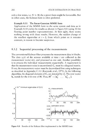
Example 8.11 The linear-Gaussian MMSE form
Application of the MMSE form to the same system and data as in
Example 8.10 yields the results as shown in Figure 8.8 (using 32-bit
floating point number representations). At first sight, there seems
nothing wrong with these results. However, the sudden change of
the smallest eigenvalue at i ¼ 2, from which point on it remains
constant, is reason to become suspicious.

8.3.2 Sequential processing of the measurements

The conventional Kalman filter processes the measurement data in blocks.
The data z n (i) of the sensors available at time i are collected in the
measurement vector z(i), and processed as one unit. Another possibility
is to process the individual measurements sequentially. A requirement is
that the measurement noise is uncorrelated. C v must be a diagonal matrix.
If not, the measurement vector must be decorrelated first using techniques
as described in Appendix C.3.1 (Kaminski et al., 1971). In the following
2
algorithm, the diagonal elements of C v are denoted by . The row vector
n
T T T
h n stands for the n-th row of H.Thus, H ¼ [ h ... h ].
0 N 1

x 10 –7 minimum eigenvalue of C(i|i)
9 15 measurements
10
8.5 5
0
8 –5
–10
0 50 100 150 200
7.5
0.04 estimation errors
7 0.02
0
6.5
–0.02
6 –0.04
0 50 100 150 200 0 50 100 150 200
i i
Figure 8.8 Results of the Kalman filter implemented in the MMSE form