Page 292 - Classification Parameter Estimation & State Estimation An Engg Approach Using MATLAB

COMPUTATIONAL ISSUES 281

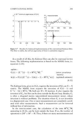
x 10 –4 minimum eigenvalue of C(i|i)
2 15 measurements
10
5
0
0
–5
2
–10
0 50 100 150 200
–4 4 estimation errors
2
–6 0
–2
8 –4
0 50 100 150 200 0 50 100 150 200
i i
Figure 8.7 Results of a balanced implementation of the conventional Kalman filter.
The filter is stable, but still an eigenvalue of C(iji) is sometimes negative

As a result of all this, the Kalman filter can also be expressed in two
forms. The following implementation is based on the MMSE form, i.e.
equation (3.20):

update :
1
1 T 1
CðijiÞ¼ C ðiji 1Þþ H C H (error covariance
v
matrixÞ
1 T 1

xðijiÞ¼ CðijiÞ C ðiji 1Þxðiji 1Þþ H C zðiÞ (updated estimate)
v
ð8:32Þ
The Kalman form, given in (8.2), requires the inversion of S(i), an N N
matrix. The MMSE form requires the inversion of C(iji 1) and
1
T
C (i 1ji) þ H C 1 H; both are M M matrices. It also requires the
v
inversion of C v , but this can be done outside the Ricatti loop. Besides, C v
is often a diagonal matrix (uncorrelated measurement noise), whose
inversion is without problems. The situation where C v is not invertible
is a degenerated case. One or more measurements are completely correl-
ated with other measurements. Such a measurement can be removed
without loss of information.
1
T
In the time-invariant case, the calculation of the term H C H,
v
appearing in (8.32), can be kept outside the loop. If so, the number of
3
2
operations is 2M þ M þ M. Thus, if there are many measurements and