Page 291 - Classification Parameter Estimation & State Estimation An Engg Approach Using MATLAB

280 STATE ESTIMATION IN PRACTICE

x 10 –6 minimum eigenvalue of C(i|i)
3 5 measurements
0
2
–5
1
–10
0 5 10 15 20 25 30 35
0
4000 estimation errors
–1
2000
–2
0
–3 –2000
0 5 10 15 20 25 30 35 0 5 10 15 20 25 30 35
i i

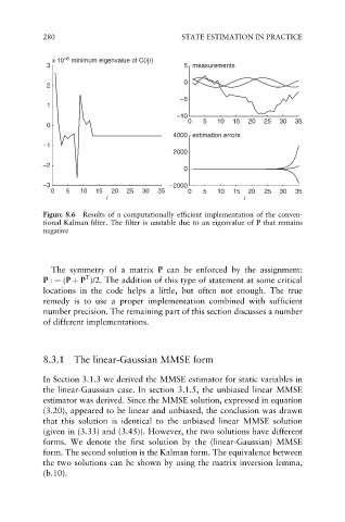
Figure 8.6 Results of a computationally efficient implementation of the conven-
tional Kalman filter. The filter is unstable due to an eigenvalue of P that remains
negative

The symmetry of a matrix P can be enforced by the assignment:
T
P : ¼ (P þ P )/2. The addition of this type of statement at some critical
locations in the code helps a little, but often not enough. The true
remedy is to use a proper implementation combined with sufficient
number precision. The remaining part of this section discusses a number
of different implementations.

8.3.1 The linear-Gaussian MMSE form

In Section 3.1.3 we derived the MMSE estimator for static variables in
the linear-Gaussian case. In section 3.1.5, the unbiased linear MMSE
estimator was derived. Since the MMSE solution, expressed in equation
(3.20), appeared to be linear and unbiased, the conclusion was drawn
that this solution is identical to the unbiased linear MMSE solution
(given in (3.33) and (3.45)). However, the two solutions have different
forms. We denote the first solution by the (linear-Gaussian) MMSE
form. The second solution is the Kalman form. The equivalence between
the two solutions can be shown by using the matrix inversion lemma,
(b.10).