Page 286 - Classification Parameter Estimation & State Estimation An Engg Approach Using MATLAB

OBSERVABILITY, CONTROLLABILITY AND STABILITY 275

0:2166 0:1624
P ¼ with eigenvalues 0 and 0:338
0:1624 0:1218
P is not invertible. The eigenvalues of F are 0.9 and 0.5. The Kalman
filter, with eigenvalues 0.5411 and 0.5, is stable.
The explanation of this behaviour is as follows. The diagonalized
system has one controllable state (corresponding to an eigenvalue of
0.9). For this state, the Kalman filter behaves regularly. The second
state (with eigenvalue 0.5) is not controllable. This state is not
affected by the process noise. It is a stable state, and thus, the initial
uncertainty fades out. The zero variance of this state causes a zero
eigenvalue in C x (1): With that, the Kalman gain for that state also
becomes zero because without uncertainty there is no need for
measurements. Consequently, the eigenvalue of the system repeats
itself in the Kalman filter. The zero eigenvalue of C x (1)causes a
corresponding zero eigenvalue in P. Thus, this matrix is not invertible.
If the second eigenvalue of F is increased from 0.5 to 1.5, the initial
condition C x (0) influences the long term behaviour of C x (i). If
C x (0) ¼ 0, then C x (i) converges to a constant. But this solution is
not stable. A small perturbation of C x (0) causes C x (i) to diverge to
infinity. Small perturbations of C x (0) trigger P(i) to follow quite
different trajectories, but they finally converge to a nonzero steady
state for which the Kalman filter is stable.

The last example shows that if a system (F, G) is not controllable,
some eigenvalues of the prediction covariance matrix may become zero.
The matrix P is positive semidefinite. Such a situation does not contrib-
ute to the numerical stability.

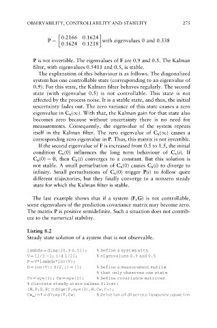
Listing 8.2
Steady state solution of a system that is not observable.

lambda ¼ diag([0.9 0.5]); % Define a system with
V ¼ [1/3 1; 1/4 1/2]; % eigenvalues 0.9 and 0.5
F ¼ V*lambda*inv(V);
H ¼ inv(V); H(2,:) ¼ []; % Define a measurement matrix
% that only observes one state
Cv ¼ eye(1); Cw ¼ eye(2); % Define covariance matrices
% Discrete steady state Kalman filter:
[M,P,Z,E] ¼ dlqe(F,eye(2),H,Cw,Cv);
Cx_inf ¼ dlyap(F,Cw) % Solution of discrete Lyapunov equation