Page 283 - Classification Parameter Estimation & State Estimation An Engg Approach Using MATLAB

272 STATE ESTIMATION IN PRACTICE

C w (i). The matrices G(i) and V w (i) are M K matrices. The introduction
of G(i) allows us to write the system equation as:

w
xði þ 1Þ¼ FðiÞxðiÞþ LðiÞuðiÞþ GðiÞ~ wðiÞ ð8:23Þ

w
where ~ w(i)isa K dimensional Gaussian white noise vector with covari-
ance matrix I. The noise sequence w(i) influences each element of x(i)
independently if the system (F(i), G(i)) is controllable by the sequence
~ w w(i). We then have the following theorem (Bar-Shalom, 1993), which
provides a sufficient (but not a necessary) condition for stability:

If a time invariant system (F, H) is completely observable and the
system (F, G) is completely controllable, then for any initial condition
P(0) ¼ C x (0) the solution of the Ricatti equation converges to a
unique, finite, invertible steady state covariance matrix P(1).

The observability of the system assures that the sequence of measure-
ments contains information about the complete state vector. Therefore,
the observability guarantees that the prediction covariance matrix P(1)
is bounded from above. Consequently, the steady state Kalman filter is
BIBO stable. See Appendix D.3.2. If one or more state elements are not
observable, the Kalman gains for these elements will be zero, and the
estimation of these elements is purely prediction driven (model based
without using measurements). If the system F is unstable for these elem-
ents, then so is the Kalman filter.
The controllability with respect ~ w(i) assures that P(1) is unique ( does
w
not depend on C x (0)), and that its inverse exists. If the system is not
controllable, then P(1) might depend on the specific choice of C x (0). If
for the non-controllable state elements the system F is stable, then the
corresponding eigenvalues of P(1) are zero. Consequently, the Kalman
gains for these elements are zero, and the estimation of these elements is
again purely prediction driven.
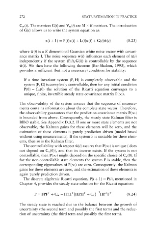
The discrete algebraic Ricatti equation, P(i þ 1) ¼ P(i), mentioned in
Chapter 4, provides the steady state solution for the Ricatti equation:

T T
T
T
P ¼ FPF þ C w FPH T HPH þ C v 1 HP F ð8:24Þ
The steady state is reached due to the balance between the growth of
uncertainty (the second term and possibly the first term) and the reduc-
tion of uncertainty (the third term and possibly the first term).