Page 285 - Classification Parameter Estimation & State Estimation An Engg Approach Using MATLAB

274 STATE ESTIMATION IN PRACTICE

(the discrete Lyapunov equation). Since the Kalman filter is optimal, the
steady state solution of the Ricatti equation is bounded from above by
C x (1), and thus asymptotical stable. The MATLAB function dlyap()
returns the solution of the discrete Lyapunov equation.

Example 8.8 Stability of a system that is not observable (continued)
A further inspection of the situation confirms the statement made
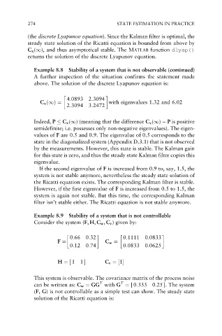
above. The solution of the discrete Lyapunov equation is:

4:0893 2:3094
C x ð1Þ ¼ with eigenvalues 1.32 and 6.02
2:3094 3:2472

Indeed, P C x (1) (meaning that the difference C x (1) P is positive
semidefinite; i.e. possesses only non-negative eigenvalues). The eigen-
values of F are 0.5 and 0.9. The eigenvalue of 0.5 corresponds to the
state in the diagonalized system (Appendix D.3.1) that is not observed
by the measurements. However, this state is stable. The Kalman gain
for this state is zero, and thus the steady state Kalman filter copies this
eigenvalue.
If the second eigenvalue of F is increased from 0.9 to, say, 1.5, the
system is not stable anymore, nevertheless the steady state solution of
the Ricatti equation exists. The corresponding Kalman filter is stable.
However, if the first eigenvalue of F is increased from 0.5 to 1.5, the
system is again not stable. But this time, the corresponding Kalman
filter isn’t stable either. The Ricatti equation is not stable anymore.

Example 8.9 Stability of a system that is not controllable
Consider the system (F, H, C w , C v ) given by:

0:66 0:32 0:1111 0:0833

F ¼ C w ¼
0:12 0:74 0:0833 0:0625

H ¼½ 11 Š C v ¼½1Š

This system is observable. The covariance matrix of the process noise
T
T
can be written as: C w ¼ GG with G ¼ [0:333 0:25 ]. The system
(F, G) is not controllable as a simple test can show. The steady state
solution of the Ricatti equation is: