Page 275 - Classification Parameter Estimation & State Estimation An Engg Approach Using MATLAB

264 STATE ESTIMATION IN PRACTICE

8.1.5 Identification of linear systems with a random input

There is a rich literature devoted to the problem of explaining a random
sequence x(i) by means of a linear system driven by white noise (Box,
1976). An example of such a model is the autoregressive model intro-
duced in Section 4.2.1. The Mth order AR model is:

M
X
xðiÞ¼ n xði nÞþ wðiÞ ð8:9Þ
n¼1

This type of model is easily cast into a state space model. As such it can
be used to describe non-white process noise. More general schemes are
the autoregressive moving average (ARMA) models and the autoregres-
sive integrating moving average (ARIMA) models. The discussion here is
only introductory and is restricted to AR models. For a full treatment we
refer to the pertinent literature.
The identification of an AR model from an observed sequence x(i)
boils down to the determination of the order M, and the estimation of
2
the parameters n and . Assuming that the system is in the steady
w
state, the estimation can be done by solving the Yule–Walker equations.
These equations arise if we multiply (8.9) on both sides by
x(i 1), .. . , x(i M), and take expectations:

M
X
½
½
E xðiÞxði kފ ¼ n E xði nÞxði kފ
n¼1 ð8:10Þ
þ E½wðiÞxði kފ for k ¼ 1; .. . ; M
def
2
Since E[x(i k)w(i)] ¼ 0 and r k ¼ E[x(i)(i k)]/ , equation (8.10)
x
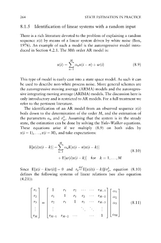
defines the following systems of linear relations (see also equation
(4.21)):

2 3 2 3 2 3
r 1 1 r 1 r 2 r M 1
1
6 7 6 1 7
r 1 r 1 r 2 6 7
6 r 2 7 6 r M 2 7
6 2 7
6 7 6 7 6 7
r 3 r 2 r 1 r 1 r M 3 6 7 ð8:11Þ
6 7 6 1 7
6 7 ¼ 6 7 3 7
6
6 . 7 6 . . . . 7
6 . 7 6 . . . . . . . . 7 6 7
5
4
4 . 5 4 5
r M r M 1 r M 2 1 M