Page 273 - Classification Parameter Estimation & State Estimation An Engg Approach Using MATLAB

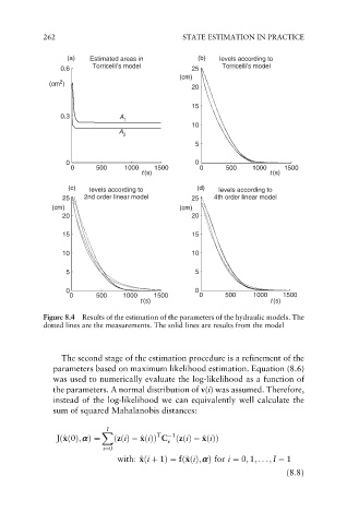
262 STATE ESTIMATION IN PRACTICE

(a) Estimated areas in (b) levels according to
0.6 Torricelli’s model 25 Torricelli’s model
(cm)
2
(cm )
20
15
0.3 A
1
10
A
2
5
0 0
0 500 1000 1500 0 500 1000 1500
t (s) t (s)
(c) levels according to (d) levels according to
25 2nd order linear model 25 4th order linear model
(cm) (cm)
20 20

15 15

10 10

5 5
0 0
0 500 1000 1500 0 500 1000 1500
t (s) t (s)
Figure 8.4 Results of the estimation of the parameters of the hydraulic models. The
dotted lines are the measurements. The solid lines are results from the model

The second stage of the estimation procedure is a refinement of the
parameters based on maximum likelihood estimation. Equation (8.6)
was used to numerically evaluate the log-likelihood as a function of
the parameters. A normal distribution of v(i) was assumed. Therefore,
instead of the log-likelihood we can equivalently well calculate the
sum of squared Mahalanobis distances:

I
X T 1
x
x
x
Jð^ xð0Þ; aÞ¼ ðzðiÞ ^ xðiÞÞ C ðzðiÞ ^ xðiÞÞ
v
i¼0
with: ^ xði þ 1Þ¼ fð^ xðiÞ; aÞ for i ¼ 0; 1; ... ; I 1
x
x
ð8:8Þ