Page 277 - Classification Parameter Estimation & State Estimation An Engg Approach Using MATLAB

266 STATE ESTIMATION IN PRACTICE

(a) (b)
1 observed signal 1.2 partial autocorrelation function
1
0.5 0.8
0.6
0
0.4
0.2
–0.5
0
–1 –0.2
0 100 200 300 400 500 0 1 2 3 4 5
i M
(c)
1 a realization of the corresponding AR process
0.5
0

–0.5
–1
0 100 200 300 400 500
i
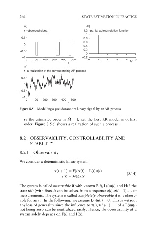
Figure 8.5 Modelling a pseudorandom binary signal by an AR process

^
M
so the estimated order is M ¼ 1, i.e. the best AR model is of first
order. Figure 8.5(c) shows a realization of such a process.

8.2 OBSERVABILITY, CONTROLLABILITY AND
STABILITY

8.2.1 Observability

We consider a deterministic linear system:

xði þ 1Þ¼ FðiÞxðiÞþ LðiÞuðiÞ
ð8:14Þ
zðiÞ¼ HðiÞxðiÞ

The system is called observable if with known F(i), L(i)u(i) and H(i) the
state x(i) (with fixed i) can be solved from a sequence z(i), z(i þ 1), .. . of
measurements. The system is called completely observable if it is observ-
able for any i. In the following, we assume L(i)u(i) ¼ 0. This is without
any loss of generality since the influence to z(i), z(i þ 1), ... of a L(i)u(i)
not being zero can be neutralized easily. Hence, the observability of a
system solely depends on F(i) and H(i).