Page 319 - Classification Parameter Estimation & State Estimation An Engg Approach Using MATLAB

308 STATE ESTIMATION IN PRACTICE

5 z(i)
4
3
2
1
0
–1
–2
–3
–4
–5
0 100 200 300 400 500 600 700 800 900 1000
i

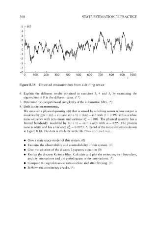
Figure 8.18 Observed measurements from a drifting sensor

6. Explain the different results obtained in exercises 3, 4 and 5, by examining the
eigenvalues of F in the different cases. (**)
7. Determine the computational complexity of the information filter. (*)
8. Drift in the measurements.
We consider a physical quantity x(i) that is sensed by a drifting sensor whose output is
v
v
modelled by z(i) ¼ x(i) þ v(i)and v(i þ 1) ¼ v(i) þ ~ v(i)with ¼ 0:999. ~ v(i) is a white
2
noise sequence with zero mean and variance ¼ 0:002. The physical quantity has a
~ v v
limited bandwidth modelled by x(i þ 1) ¼ x(i) þ w(i)with ¼ 0:95. The process
2
noise is white and has a variance ¼ 0:0975. A record of the measurements is shown
w
in Figure 8.18. The data is available in the file C8exercise8:mat.
. Give a state space model of this system. (0)
. Examine the observability and controllability of this system. (0)
. Give the solution of the discrete Lyapunov equation (0)
. Realize the discrete Kalman filter. Calculate and plot the estimates, its boundary,
and the innovations and the periodogram of the innovations. (*)
. Compare the signal-to-noise ratios before and after filtering. (0)
. Perform the consistency checks. (*)