Page 315 - Classification Parameter Estimation & State Estimation An Engg Approach Using MATLAB

304 STATE ESTIMATION IN PRACTICE

measurements, we have recorded a set of measurements Z K ¼fz(0),
z(1), .. . , z(K)g. Using the prior knowledge E[x(0)] and C x (0) we want
estimates for some points in time 0 k K. We emphasize once again
that this section is only introductory. For details we refer to the pertinent
literature (Gelb et al., 1974).
The problem is often divided into three types of problems:

. Fixed interval smoothing: K is fixed. k is variable between 0 and K.
. Fixed point smoothing: k is fixed. K increases with time, K ¼ i.
. Fixed lag smoothing: both k and K increase with time, but with
def
K k fixed to the so-called lag¼ K k. Thus, K ¼ i and
k ¼ i lag.

Fixed interval smoothing is needed most often. The problem occurs
when an experiment has been done, the data has been acquired and
stored, and the data is analysed afterwards.
The general approach to smoothing is the same as for discrete states.
See Section 4.3.3. The estimation occurs in two passes. In the first pass,
the data is processed forward in time to yield estimates ^ x f (k) ¼ x(kjk). In
x
the second pass, the data is processed backward in time. Starting with
k ¼ K we recursively estimate the previous states using only data from
x
the ‘future’. Thus, the backward estimate ^ x b (k) only uses information
from Z K Z kþ1 ¼fz(k þ 1), .. . , z(K)g. For that, a ‘reversed time’
Kalman filter can be used. The final estimate x(kjK) is obtained by
x
optimally combining ^ x f (k) and ^ x b (k).
x
Although this approach yields the desired optimally smoothed states, it is
not computationally efficient. For each of the three differenttypes ofsmooth-
ing problems more efficient algorithms have been proposed. One of them is
the well-known Rauch–Tung–Striebel smoother (Rauch etal., 1965). The
algorithm implements a fixed interval smoother. It does not explicitly use
^ x x b (k). Instead, it uses recursively x(kjK). The algorithm is as follows:

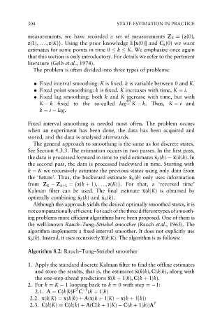
Algorithm 8.2: Rauch–Tung–Striebel smoother

1. Apply the standard discrete Kalman filter to find the offline estimates
and store the results, that is, the estimates x(kjk), C(kjk), along with
the one-step-ahead predictions x(k þ 1jk), C(k þ 1jk).
2. For k ¼ K 1 looping back to k ¼ 0 with step ¼ 1:
1
T
2.1. A ¼ C(kjk)F C (k þ 1jk)
2.2. x(kjK) ¼ x(kjk) þ A(x(k þ 1jK) x(k þ 1jk))
2.3. C(kjK) ¼ C(kjk) þ A(C(k þ 1jK) C(k þ 1jk))A T