Page 312 - Classification Parameter Estimation & State Estimation An Engg Approach Using MATLAB

EXTENSIONS OF THE KALMAN FILTER 301

The new, augmented state vector can be estimated using the standard
Kalman filter.
The case of autocorrelated measurement noise is handled in the same
way although some complications may occur (Bryson and Hendrikson,
1965). Suppose that the measurement noise is modelled by
v
v
v(i þ 1) ¼ F v v(i) þ ~ v(i) with ~ v(i) a white noise sequence with covariance
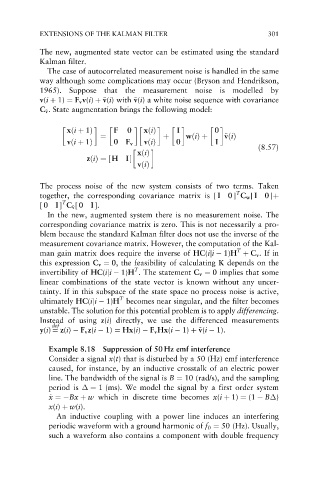
C ~ v . State augmentation brings the following model:
v

xði þ 1Þ F 0 xðiÞ I 0
¼ þ wðiÞþ ~ v vðiÞ
vði þ 1Þ 0F v vðiÞ 0 I
ð8:57Þ

xðiÞ
zðiÞ¼ H I Š
½
vðiÞ
The process noise of the new system consists of two terms. Taken
T
together, the corresponding covariance matrix is [ I 0 ] C w [ I 0 ]þ
T
[ 0I ] C ~ v [ 0I ].
v
In the new, augmented system there is no measurement noise. The
corresponding covariance matrix is zero. This is not necessarily a pro-
blem because the standard Kalman filter does not use the inverse of the
measurement covariance matrix. However, the computation of the Kal-
T
man gain matrix does require the inverse of HC(iji 1)H þ C v .If in
this expression C v ¼ 0, the feasibility of calculating K depends on the
T
invertibility of HC(iji 1)H . The statement C v ¼ 0 implies that some
linear combinations of the state vector is known without any uncer-
tainty. If in this subspace of the state space no process noise is active,
T
ultimately HC(iji 1)H becomes near singular, and the filter becomes
unstable. The solution for this potential problem is to apply differencing.
Instead of using z(i) directly, we use the differenced measurements
def
v
y(i) ¼ z(i) F v z(i 1) ¼ Hx(i) F v Hx(i 1) þ ~ v(i 1).
Example 8.18 Suppression of 50 Hz emf interference
Consider a signal x(t) that is disturbed by a 50 (Hz) emf interference
caused, for instance, by an inductive crosstalk of an electric power
line. The bandwidth of the signal is B ¼ 10 (rad/s), and the sampling
period is ¼ 1 (ms). We model the signal by a first order system
_ x x ¼ Bx þ w which in discrete time becomes x(i þ 1) ¼ (1 B )
x(i) þ w(i).
An inductive coupling with a power line induces an interfering
periodic waveform with a ground harmonic of f 0 ¼ 50 (Hz). Usually,
such a waveform also contains a component with double frequency