Page 311 - Classification Parameter Estimation & State Estimation An Engg Approach Using MATLAB

300 STATE ESTIMATION IN PRACTICE

covariance matrix C w of the process noise by means of a fudge factor
.
For instance, we simply replace C w by C w þ
I. Other methods to
regulate a covariance matrix are discussed in Section 5.2.3. Instead of
adapting C w we can also increase the diagonal of the prediction covari-
ance C(i þ 1ji) by some factor. The fudge factor should be selected such
that the consistency checks now pass as successful as possible.
Fudging effectuates a decreaseoffaith in the modelofthe process, andthus
causes a larger impact of the measurements. However, modelling errors give
rise to deviations that are autocorrelated and not independent from the
states. Thus, these deviations are not accurately modelled by white noise.
The designer should maintain a critical attitude with respect to fudging.

8.5 EXTENSIONS OF THE KALMAN FILTER

The extensions considered in this section make the Kalman filter applic-
able to a wider class of problems. In particular, we discuss extensions to
cover non-white and cross-correlated noise sequences. Also, the topic of
offline estimation will be introduced.

8.5.1 Autocorrelated noise

The Kalman filter considered so far assumes white uncorrelated random
sequences w(i) and v(i) for the process and measurement noise. What do
we do if these assumptions do not hold in practice?
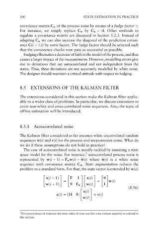
The case of autocorrelated noise is usually tackled by assuming a state
3
space model for the noise. For instance, autocorrelated process noise is
w
w
represented by w(i þ 1) ¼ F w w(i) þ ~ w(i) where ~ w(i) is a white noise
sequence with covariance matrix C ~ w . State augmentation reduces the
w
problem to a standard form. For that, the state vector is extended by w(i):
" # " #" # "#
xði þ 1Þ F I xðiÞ 0
¼ þ ~ w wðiÞ
wði þ 1Þ 0F w wðiÞ I
ð8:56Þ
" #
xðiÞ
zðiÞ¼ H 0 Š þ vðiÞ
½
wðiÞ

3
For convenience of notation the time index of matrices (for time variant systems) is omitted in
this section.