Page 313 - Classification Parameter Estimation & State Estimation An Engg Approach Using MATLAB

302 STATE ESTIMATION IN PRACTICE

(and possibly higher harmonics, but these will be neglected here). The
disturbance can be modelled by two second order equations, that is:

2 3
cosð2 f 0 Þ sinð2 f 0 Þ
0
6 7
sinð2 f 0 Þ cosð2 f 0 Þ
v
6 7
7vðiÞþ ~ vðiÞ
vði þ 1Þ¼ d6
cosð4 f 0 Þ
4 sinð4 f 0 Þ 5
0
sinð4 f 0 Þ cosð4 f 0 Þ
ð8:58Þ
The factor d is selected close to one, modelling the fact that the
magnitudes of each component vary in time only slowly.
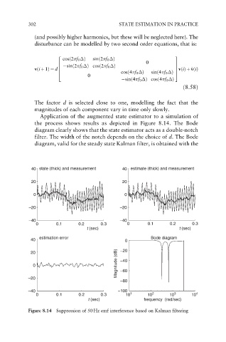
Application of the augmented state estimator to a simulation of
the process shows results as depicted in Figure 8.14. The Bode
diagram clearly shows that the state estimator acts as a double-notch
filter. The width of the notch depends on the choice of d.The Bode
diagram, valid for the steady state Kalman filter, is obtained with the

40 state (thick) and measurement 40 estimate (thick) and measurement

20 20

0 0

–20 –20

–40 –40
0 0.1 0.2 0.3 0 0.1 0.2 0.3
t (sec) t (sec)
estimation error Bode diagram
40 0
Magnitude (dB) –40
20 –20
0 –60

–20
–80
–40 –100
0 0.1 0.2 0.3 10 1 10 2 10 3 10 4
t (sec) frequency (rad/sec)

Figure 8.14 Suppression of 50 Hz emf interference based on Kalman filtering