Page 318 - Classification Parameter Estimation & State Estimation An Engg Approach Using MATLAB

EXERCISES 307

8.7 EXERCISES

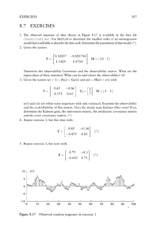
1. The observed sequence of data shown in Figure 8.17 is available in the data file
C8exercise1:mat.Use MATLAB to determine the smallest order of an autoregressive
modelthatis stillabletodescribethedatawell.Determinetheparameters ofthatmodel.(*).
2. Given the system:

" #
0:32857 0:085714
½
F ¼ H ¼ 10 5 Š
1:1429 1:0714
Determine the observability Grammian and the observability matrix. What are the
eigenvalues of these matrices? What can be said about the observability? (0)
3. Given the system x(i þ 1) ¼ Fx(i) þ Gw(i) and z(i) ¼ Hx(i) þ v(i) with

" #
0:65 0:06 2
F ¼ G ¼ H ¼ 1 1 Š
½
0:375 0:65 5
w(i) and v(i) are white noise sequences with unit variances. Examine the observability
and the controllability of this system. Does the steady state Kalman filter exist? If so,
determine the Kalman gain, the innovation matrix, the prediction covariance matrix
and the error covariance matrix. (*)
4. Repeat exercise 3, but this time with:

" #
0:85 0:14
F ¼ ð*Þ
0:875 0:85
5. Repeat exercise 3, but now with:

" #
0:75 0:1
F ¼ ð*Þ
0:625 0:75

10 x(i)

5

0
–5

–10
0 10 20 30 40 50 60 70 80 90 100
i
Figure 8.17 Observed random sequence in exercise 1