Page 322 - Classification Parameter Estimation & State Estimation An Engg Approach Using MATLAB

BOSTON HOUSING CLASSIFICATION PROBLEM 311

ignore this problem, and we will assume that all features are real valued.
(Obviously, we will lose some performance using this assumption.)

9.1.2 Simple classification methods

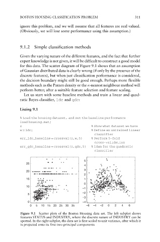
Given the varying nature of the different features, and the fact that further
expert knowledge is not given, it will be difficult to construct a good model
for this data. The scatter diagram of Figure 9.1 shows that an assumption
of Gaussian distributed data is clearly wrong (if only by the presence of the
discrete features), but when just classification performance is considered,
the decision boundary might still be good enough. Perhaps more flexible
methods such as the Parzen density or the -nearest neighbour method will
perform better; after a suitable feature selection and feature scaling.
Let us start with some baseline methods and train a linear and quad-
ratic Bayes classifier, ldc and qdc:

Listing 9.1

% Load the housing dataset, and set the baseline performance
load housing.mat;
z % Show what dataset we have
w ¼ ldc; % Define an untrained linear
classifier
err_ldc_baseline ¼ crossval(z,w,5) % Perform 5-fold
cross-validation
err_qdc_baseline ¼ crossval(z,qdc,5) % idem for the quadratic
classifier

5
25
4
3
20
2
15 1
0
10
–1
–2
5
–3
0 –4
0 5 10 15 20 25 30 35 –6 –4 –2 0 2 4 6

Figure 9.1 Scatter plots of the Boston Housing data set. The left subplot shows
features STATUS and INDUSTRY, where the discrete nature of INDUSTRY can be
spotted. In the right subplot, the data set is first scaled to unit variance, after which it
is projected onto its first two principal components