Page 321 - Classification Parameter Estimation & State Estimation An Engg Approach Using MATLAB

310 WORKED OUT EXAMPLES

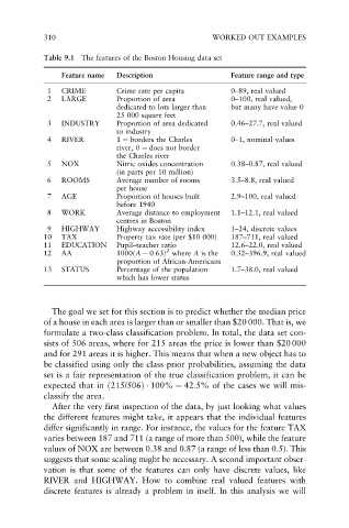
Table 9.1 The features of the Boston Housing data set

Feature name Description Feature range and type

1 CRIME Crime rate per capita 0–89, real valued
2 LARGE Proportion of area 0–100, real valued,
dedicated to lots larger than but many have value 0
25 000 square feet
3 INDUSTRY Proportion of area dedicated 0.46–27.7, real valued
to industry
4 RIVER 1 ¼ borders the Charles 0–1, nominal values
river, 0 ¼ does not border
the Charles river
5 NOX Nitric oxides concentration 0.38–0.87, real valued
(in parts per 10 million)
6 ROOMS Average number of rooms 3.5–8.8, real valued
per house
7 AGE Proportion of houses built 2.9–100, real valued
before 1940
8 WORK Average distance to employment 1.1–12.1, real valued
centres in Boston
9 HIGHWAY Highway accessibility index 1–24, discrete values
10 TAX Property tax rate (per $10 000) 187–711, real valued
11 EDUCATION Pupil–teacher ratio 12.6–22.0, real valued
2
12 AA 1000ðA 0:63Þ where A is the 0.32–396.9, real valued
proportion of African-Americans
13 STATUS Percentage of the population 1.7–38.0, real valued
which has lower status

The goal we set for this section is to predict whether the median price
of a house in each area is larger than or smaller than $20 000. That is, we
formulate a two-class classification problem. In total, the data set con-
sists of 506 areas, where for 215 areas the price is lower than $20 000
and for 291 areas it is higher. This means that when a new object has to
be classified using only the class prior probabilities, assuming the data
set is a fair representation of the true classification problem, it can be
expected that in ð215/506Þ 100% ¼ 42:5% of the cases we will mis-
classify the area.
After the very first inspection of the data, by just looking what values
the different features might take, it appears that the individual features
differ significantly in range. For instance, the values for the feature TAX
varies between 187 and 711 (a range of more than 500), while the feature
values of NOX are between 0.38 and 0.87 (a range of less than 0.5). This
suggests that some scaling might be necessary. A second important obser-
vation is that some of the features can only have discrete values, like
RIVER and HIGHWAY. How to combine real valued features with
discrete features is already a problem in itself. In this analysis we will