Page 325 - Classification Parameter Estimation & State Estimation An Engg Approach Using MATLAB

314 WORKED OUT EXAMPLES

PCA preprocessing is applied such that 90% of the variance is retained,
the performance of all the methods significantly decreases. To avoid this
clearly undesired effect, we will first rescale the data to have unit
variance and apply PCA on the resulting data. The basic training proced-
ure now becomes:

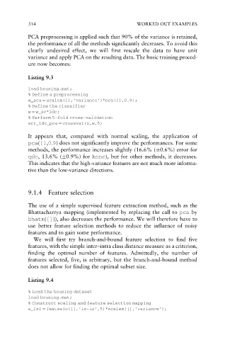
Listing 9.3

load housing.mat;
% Define a preprocessing
w_pca ¼ scalem([],‘variance’)*pca([],0.9);
% Define the classifier
w ¼ w_sc*ldc;
% Perform 5-fold cross-validation
err_ldc_pca ¼ crossval(z,w,5)

It appears that, compared with normal scaling, the application of
pca([],0:9) does not significantly improve the performances. For some
methods, the performance increases slightly (16.6% ( 0:6%) error for
qdc, 13.6% ( 0:9%) for knnc), but for other methods, it decreases.
This indicates that the high-variance features are not much more informa-
tive than the low-variance directions.

9.1.4 Feature selection

The use of a simple supervised feature extraction method, such as the
Bhattacharrya mapping (implemented by replacing the call to pca by
bhatm([])), also decreases the performance. We will therefore have to
use better feature selection methods to reduce the influence of noisy
features and to gain some performance.
We will first try branch-and-bound feature selection to find five
features, with the simple inter–intra class distance measure as a criterion,
finding the optimal number of features. Admittedly, the number of
features selected, five, is arbitrary, but the branch-and-bound method
does not allow for finding the optimal subset size.

Listing 9.4

% Load the housing dataset
load housing.mat;
% Construct scaling and feature selection mapping
w_fsf ¼ featselo([],‘in-in’,5)*scalem([],‘variance’);