Page 328 - Classification Parameter Estimation & State Estimation An Engg Approach Using MATLAB

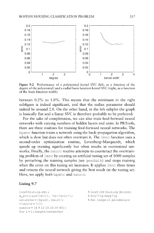
BOSTON HOUSING CLASSIFICATION PROBLEM 317

0.2 0.2
0.18 0.18
0.16 0.16
0.14 0.14
0.12 0.12
error 0.1 error 0.1
0.08 0.08
0.06 0.06
0.04 0.04
0.02 0.02
0 0
1 2 3 0 1 2 3 4
degree kernel width
Figure 9.2 Performance of a polynomial kernel SVC (left, as a function of the
degree of the polynomial) and a radial basis function kernel SVC (right, as a function
of the basis function width)

between 0.2% to 1.0%. This means that the minimum in the right
subfigure is indeed significant, and that the radius parameter should
indeed be around 2.0. On the other hand, in the left subplot the graph
is basically flat and a linear SVC is therefore probably to be preferred.
For the sake of completeness, we can also train feed-forward neural
networks with varying numbers of hidden layers and units. In PRTools,
there are three routines for training feed-forward neural networks. The
bpxnc function trains a network using the back-propagation algorithm,
which is slow but does not often overtrain it. The lmnc function uses a
second-order optimization routine, Levenberg–Marquardt, which
speeds up training significantly but often results in overtrained net-
works. Finally, the neurc routine attempts to counteract the overtrain-
ing problem of lmnc by creating an artificial tuning set of 1000 samples
by perturbing the training samples (see gendatk) and stops training
when the error on this tuning set increases. It applies lmnc three times
and returns the neural network giving the best result on the tuning set.
Here, we apply both bpxnc and neurc:

Listing 9.7

load housing.mat; % Load the housing dataset
w_pre ¼ scalem([], ‘variance’); % Scaling mapping
networks ¼ {bpxnc, neurc}; % Set range of parameters
nlayers ¼ 1:2;
nunits ¼ [4 8 12 16 20 30 40];
for i ¼ 1:length(networks)