Page 327 - Classification Parameter Estimation & State Estimation An Engg Approach Using MATLAB

316 WORKED OUT EXAMPLES

increase in error of about 0.005. Nevertheless, feature selection in gen-
eral does not seem to help much for this data set.

9.1.5 Complex classifiers

The fact that ldc already performs so well on the original data indicates
that the data is almost linearly separable. A visual inspection of the
scatter plots in Figure 9.1 seems to strengthen this hypothesis. It becomes
even more apparent after the training of a linear support vector classifier
(svc([],‘p’,1)) and a Fisher classifier (fisherc), both with a cross-
validation error of 13.0%, the same as for ldc.
Given that ldc and parzenc thus far performed best, we might try
to train a number of classifiers based on these concepts, for which we are
able to tune classifier complexity. Two obvious choices for this are
neural networks and support vector classifiers (SVCs). Starting with
the latter, we can train SVCs with polynomial kernels of degree close
to 1, and with radial basis kernels of radius close to 1. By varying the
degree or radius, we can vary the resulting classifier’s nonlinearity:

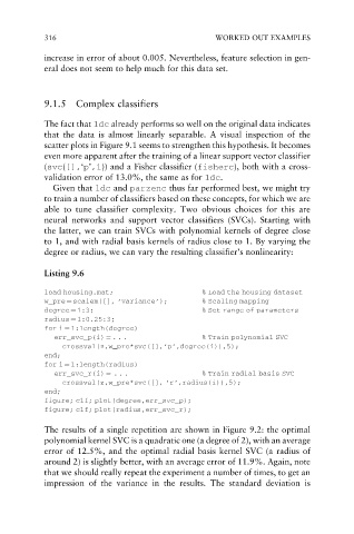
Listing 9.6

load housing.mat; % Load the housing dataset
w_pre ¼ scalem([], ‘variance’); % Scaling mapping
degree ¼ 1:3; % Set range of parameters
radius ¼ 1:0.25:3;
for i ¼ 1:length(degree)
err_svc_p(i) ¼ . . . % Train polynomial SVC
crossval(z,w_pre*svc([],‘p’,degree(i)),5);
end;
for i ¼ 1:length(radius)
err_svc_r(i) ¼ . . . % Train radial basis SVC
crossval(z,w_pre*svc([], ‘r’,radius(i)),5);
end;
figure; clf; plot(degree,err_svc_p);
figure; clf; plot(radius,err_svc_r);

The results of a single repetition are shown in Figure 9.2: the optimal
polynomial kernel SVC is a quadratic one (a degree of 2), with an average
error of 12.5%, and the optimal radial basis kernel SVC (a radius of
around 2) is slightly better, with an average error of 11.9%. Again, note
that we should really repeat the experiment a number of times, to get an
impression of the variance in the results. The standard deviation is