Page 329 - Classification Parameter Estimation & State Estimation An Engg Approach Using MATLAB

318 WORKED OUT EXAMPLES

for j ¼ 1:length(nlayers)
for k ¼ 1:length(nunits)
% Train a neural network with nlayers(j) hidden layers
% of nunits(k) units each, using algorithm network{i}
err_nn(i,j,k) ¼ crossval(z, . . .
w_pre*networks{i}([],ones(1,nlayers(j))*nunits(k)),5);
end;
end;
figure; clear all; % Plot the errors
plot(nunits,err_nn(i,1,:), ‘-’); hold on;
plot(nunits,err_nn(i,2,:), ‘--’);
legend(‘1 hidden layer’, ‘2 hidden layers’);
end;

Training neural networks is a computationally intensive process; and
here they are trained for a large range of parameters, using cross-validation.
The algorithm above takes more than a day to finish on a modern
workstation, although per setting just a single neural network is trained.
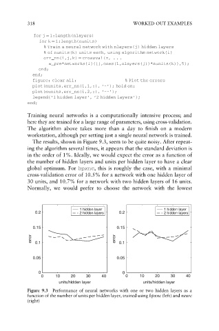
The results, shown in Figure 9.3, seem to be quite noisy. After repeat-
ing the algorithm several times, it appears that the standard deviation is
in the order of 1%. Ideally, we would expect the error as a function of
the number of hidden layers and units per hidden layer to have a clear
global optimum. For bpxnc, this is roughly the case, with a minimal
cross-validation error of 10.5% for a network with one hidden layer of
30 units, and 10.7% for a network with two hidden layers of 16 units.
Normally, we would prefer to choose the network with the lowest

1 hidden layer 1 hidden layer
0.2 2 hidden layers 0.2 2 hidden layers

0.15 0.15
error 0.1 error 0.1

0.05 0.05

0 0
0 10 20 30 40 0 10 20 30 40
units/hidden layer units/hidden layer
Figure 9.3 Performance of neural networks with one or two hidden layers as a
function of the number of units per hidden layer, trained using bpxnc (left) and neurc
(right)