Page 333 - Classification Parameter Estimation & State Estimation An Engg Approach Using MATLAB

322 WORKED OUT EXAMPLES

nominal response h(t), but now time-shifted by t and attenuated by a.
Such an assumption is correct for a medium like air because, within the
bandwidth of interest, the propagation of a waveform through air does
not show a significant dispersion. The attenuation coefficient a depends
on many factors, but also on the distance, and thus also on t. However,
for the moment we will ignore this fact. The possible echoes are
represented by a r(t t). They share the same time shift t because no
echo can occur before the arrival of the nominal response. The addi-
tional time delays of the echoes are implicitly modelled within r(t). The
echoes and the nominal response also share a common attenuation
factor. The noise v(t) is considered white.
The actual shape of the nominal response h(t) depends on the choice
of the tone burst and on the dynamic properties of the transducers.
Sometimes, a parametric empirical model is used, for instance:

m
hðtÞ¼ t expð t=TÞ cosð2 ft þ ’Þ t 0 ð9:2Þ
f is the frequency of the tone burst; cos (2 ft þ ’) is the carrier; and
m
t exp ( t/T) is the envelope. The factor t m describes the rise of the
waveform (m is empirically determined; usually between 1 and 3). The
factor exp ( t/T) describes the decay. Another possibility is to model h(t)
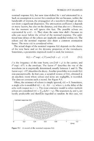
non-parametrically. In that case, a sampled version of h(t), obtained in
an anechoic room where echoes and noise are negligible, is recorded.
The data set contains such a record. See Figure 9.5.
Often, the existence of echoes is simply ignored, r(t) ¼ 0. Sometimes,
a single echo is modelled r(t) ¼ d 1 h(t t 1 ) where t 1 is the delay of the
echo with respect to t ¼ t. The most extensive model is when multiple
P
echoes are considered r(t) ¼ k d k h(t t k ). The sequences d k and t k are
hardly predictable and therefore regarded as random. In that case, r(t)

nominal response h(t)

0 0.2 0.4 0.6 0.8 1 1.2
t(ms)
Figure 9.5 A record of the nominal response h(t)