Page 336 - Classification Parameter Estimation & State Estimation An Engg Approach Using MATLAB

TIME-OF-FLIGHT ESTIMATION OF AN ACOUSTIC TONE BURST 325

noise sensitivity is large. If the interval is too large, modelling errors
become too influential. The strategy is to find two anchor points t 1 and
t 2 that are stable enough under the various conditions.
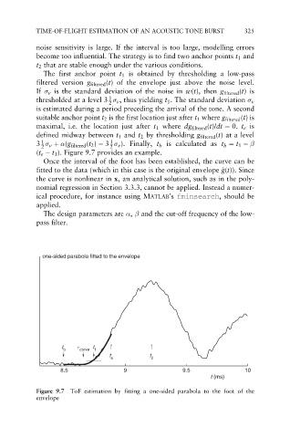
The first anchor point t 1 is obtained by thresholding a low-pass
filtered version g filtered (t) of the envelope just above the noise level.
If v is the standard deviation of the noise in w(t), then g filtered (t)is
1
thresholded at a level 3 v , thus yielding t 1 . The standard deviation v
2
is estimated during a period preceding the arrival of the tone. A second
suitable anchor point t 2 is the first location just after t 1 where g filtered (t)is
maximal, i.e. the location just after t 1 where dg filtered (t)/dt ¼ 0. t e is
defined midway between t 1 and t 2 by thresholding g filtered (t) at a level
1
1
3 v þ (g filtered (t 2 ) 3 v ). Finally, t b is calculated as t b ¼ t 1
2 2
(t e t 1 ). Figure 9.7 provides an example.
Once the interval of the foot has been established, the curve can be
fitted to the data (which in this case is the original envelope ^ g(t)). Since
g
the curve is nonlinear in x, an analytical solution, such as in the poly-
nomial regression in Section 3.3.3, cannot be applied. Instead a numer-
ical procedure, for instance using MATLAB’s fminsearch, should be
applied.
The design parameters are , and the cut-off frequency of the low-
pass filter.

one-sided parabola fitted to the envelope

t τ t
b curve 1
t t
e 2
8.5 9 9.5 10
t (ms)

Figure 9.7 ToF estimation by fitting a one-sided parabola to the foot of the
envelope