Page 306 - Classification Parameter Estimation & State Estimation An Engg Approach Using MATLAB

CONSISTENCY CHECKS 295

In the linear-Gaussian case, the NEES has a 2 M distribution (chi-square
with M degrees of freedom; see Appendix C.1.5).
The 2 distribution of the NEES follows from the following
M
argument. Since the state estimator is unbiased, E[e(iji)] ¼ 0.The
covariance matrix of e(iji)is C(iji). Suppose A(i) is a symmetric
1
T
matrix such that A(i)A (i) ¼ C (iji). Application of A(i)to e(i)will
give a random vector y(i) ¼ A(i)e(i). The covariance matrix of y(i)is:
T
T
1
T
A(i)C(iji)A (i) ¼ A(i)(A(i)A (i)) A (i) ¼ I. Thus, the components of
y(i) are uncorrelated, and have unit variance. If both the process
noise and the measurement noise are normally distributed, then so
1
T
T
is y(i). Hence, the inner product y (i)y(i) ¼ e (i)C (iji)e(i)is the sum
of M squared, independent random variables, each normally
distributed with zero mean and unit variance. Such a sum has a 2 M
distribution.
The NIS (normalized innovation squared) is a test signal defined as:
T
1
z
z
NisðiÞ¼ ~ z ðiÞS ðiÞ~ zðiÞ ð8:53Þ
2
In the linear-Gaussian case, the NIS has a distribution. This follows
N
readily from the same argument as used above.
Example 8.15 Normalized errors of second order system
Consider the following system:

0:999 cosð0:1 Þ 0:999 sinð0:1 Þ
F ¼ H ¼ 00:5 Š
½
0:999 sinð0:1 Þ 0:999 cosð0:1 Þ
10

C w ¼ C v ¼½1Š ð8:54Þ
00
0:01 0 0

C x ð0Þ¼ E½xð0ފ ¼
0 0:01 0
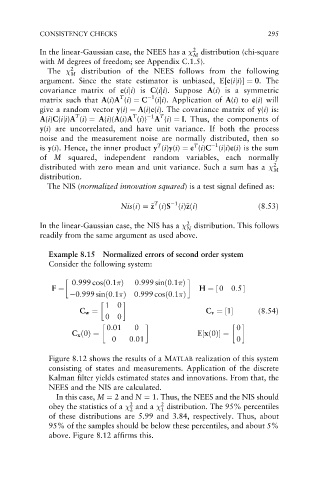
Figure 8.12 shows the results of a MATLAB realization of this system
consisting of states and measurements. Application of the discrete
Kalman filter yields estimated states and innovations. From that, the
NEES and the NIS are calculated.
In this case, M ¼ 2 and N ¼ 1. Thus, the NEES and the NIS should
2
2
obey the statistics of a and a distribution. The 95% percentiles
2 1
of these distributions are 5.99 and 3.84, respectively. Thus, about
95% of the samples should be below these percentiles, and about 5%
above. Figure 8.12 affirms this.