Page 305 - Classification Parameter Estimation & State Estimation An Engg Approach Using MATLAB
P. 305
294 STATE ESTIMATION IN PRACTICE
def
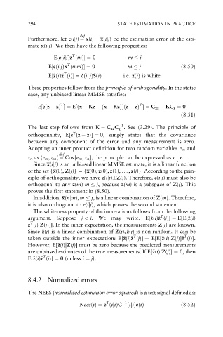
Furthermore, let e(ijj) ¼ x(i) x(ijj) be the estimation error of the esti-
mate x(ijj). We then have the following properties:
T
E½eðijjÞz ðmÞ ¼ 0 m j
T
E½eðijjÞx ðnjmÞ ¼ 0 m j ð8:50Þ
T
z
z
z
E½~ zðiÞ~ z ðjÞ ¼ ði; jÞSðiÞ i:e: ~ zðiÞ is white
These properties follow from the principle of orthogonality. In the static
case, any unbiased linear MMSE satisfies:
T
T
E½eðz zÞ ¼ E½ðx Kz ðx KzÞÞðz zÞ ¼ C xz KC z ¼ 0
ð8:51Þ
1
The last step follows from K ¼ C xz C . See (3.29). The principle of
z
T
orthogonality, E[e (z z)] ¼ 0, simply states that the covariance
between any component of the error and any measurement is zero.
Adopting an inner product definition for two random variables e m and
def
z n as (e m , z m ) ¼ Cov[e m , z n ], the principle can be expressed as e?z.
Since x(ijj) is an unbiased linear MMSE estimate, it is a linear function
of the set fx(0), Z(j)g¼ fx(0), z(0), z(1), .. . , z(j)g. According to the prin-
ciple of orthogonality, we have e(ijj)?Z(j). Therefore, e(ijj) must also be
orthogonal to any z(m) m j, because z(m) is a subspace of Z(j). This
proves the first statement in (8.50).
In addition, x(njm), m j, is a linear combination of Z(m). Therefore,
it is also orthogonal to e(ijj), which proves the second statement.
The whiteness property of the innovations follows from the following
T
z
argument. Suppose j < i. We may write: E[~ z(i)~ z (j)] ¼ E[E[~ z(i)
z
z
z T
~ z (j)jZ(j)]]. In the inner expectation, the measurements Z(j) are known.
z
z
Since ~ z(j) is a linear combination of Z(j),~ z(j) is non-random. It can be
T
T
z
z
z
z
taken outside the inner expectation: E[~ z(i)~ z (j)] ¼ E[E[~ z(i)jZ(j)]~ z (j)].
However, E[~ z(i)jZ(j)] must be zero because the predicted measurements
z
z
are unbiased estimates of the true measurements. If E[~ z(i)jZ(j)] ¼ 0, then
T
z
E[~ z(i)~ z (j)] ¼ 0 (unless i ¼ j).
z
8.4.2 Normalized errors
The NEES (normalized estimation error squared) is a test signal defined as:
T 1
NeesðiÞ¼ e ðijiÞC ðijiÞeðiÞ ð8:52Þ

