Page 300 - Classification Parameter Estimation & State Estimation An Engg Approach Using MATLAB

COMPUTATIONAL ISSUES 289

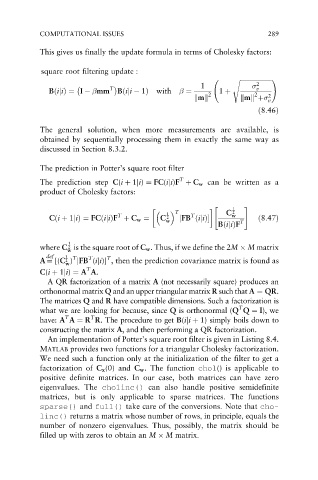
This gives us finally the update formula in terms of Cholesky factors:

square root filtering update :
s ffiffiffiffiffiffiffiffiffiffiffiffiffiffiffiffiffiffiffiffi !
1 2

BðijiÞ¼ I mm T Bðiji 1Þ with ¼ 2 1 þ 2 v
m þ
m
kk kk 2 v
ð8:46Þ
The general solution, when more measurements are available, is
obtained by sequentially processing them in exactly the same way as
discussed in Section 8.3.2.

The prediction in Potter’s square root filter
T
The prediction step C(i þ 1ji) ¼ FC(iji)F þ C w can be written as a
product of Cholesky factors:

1
" #

T C 2
T 1 T w
2
Cði þ 1jiÞ¼ FCðijiÞF þ C w ¼ C w jFB ðijiފ ð8:47Þ
BðijiÞF T
1
where C is the square root of C w . Thus, if we define the 2M M matrix
2
w
def 1
T
T
T
A ¼ [(C ) jFB (iji)] , then the prediction covariance matrix is found as
2
w
T
C(i þ 1ji) ¼ A A.
AQRfactorization of amatrix A (not necessarily square) produces an
orthonormal matrix Q and an upper triangular matrix R such that A ¼ QR.
The matrices Q and R have compatible dimensions. Such a factorization is
T
what we are looking for because, since Q is orthonormal (Q Q ¼ I), we
T
T
have: A A ¼ R R. The procedure to get B(iji þ 1) simply boils down to
constructing the matrix A, and then performing a QR factorization.
An implementation of Potter’s square root filter is given in Listing 8.4.
MATLAB provides two functions for a triangular Cholesky factorization.
We need such a function only at the initialization of the filter to get a
factorization of C x (0) and C w . The function chol() is applicable to
positive definite matrices. In our case, both matrices can have zero
eigenvalues. The cholinc() can also handle positive semidefinite
matrices, but is only applicable to sparse matrices. The functions
sparse() and full() take care of the conversions. Note that cho-
linc() returns a matrix whose number of rows, in principle, equals the
number of nonzero eigenvalues. Thus, possibly, the matrix should be
filled up with zeros to obtain an M M matrix.