Page 301 - Classification Parameter Estimation & State Estimation An Engg Approach Using MATLAB

290 STATE ESTIMATION IN PRACTICE

The QR factorization in the prediction step is taken care of by qr().
The size of the resulting matrix is (M þ K) M where K is the number of
rows in SqCw. Only the first M rows carry the needed information and
the remaining rows are deleted.
2
3
The update of the algorithm requires N(M þ 3M þ M) operations.
The number of operations of the prediction is determined partly by qr ().
3
1
2
This function requires about M þ M K operations. In full, the predic-
2
2
3
3
tion requires M þ M K operations.
2
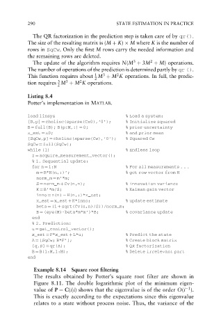
Listing 8.4
Potter’s implementation in MATLAB.
load linsys % Load a system:
[B,p] ¼ cholinc(sparse(Cx0),‘0’); % Initialize squared
B ¼ full(B); B(p:M,:) ¼ 0; % prior uncertainty
x_est ¼ x0; % and prior mean
[SqCw,p] ¼ cholinc(sparse(Cw),‘0’); % Squared Cw
SqCw ¼ full(SqCw);
while (1) % Endless loop
z ¼ acquire_measurement_vector();
% 1. Sequential update:
for n ¼ 1:N % For all measurements . . .
m ¼ B*H(n,:)’; % get row vector from H
norm_m ¼ m’*m;
S ¼ norm_m þ Cv(n,n); % innovation variance
K ¼ B’*m/S; % Kalman gain vector
inno ¼ z(n) H(n,:)*x_est;
x_est ¼ x_est þ K*inno; % update estimate
beta ¼ (1 þ sqrt(Cv(n,n)/S))/norm_m;
B ¼ (eye(M)-beta*m*m’)*B; % covariance update
end
% 2. Prediction:
u ¼ get_control_vector();
x_est ¼ F*x_est þ L*u; % Predict the state
A ¼ [SqCw; B*F’]; % Create block matrix
[q,B] ¼ qr(A); % QR factorization
B ¼ B(1:M,1:M); % Delete irrelevant part
end

Example 8.14 Square root filtering
The results obtained by Potter’s square root filter are shown in
Figure 8.11. The double logarithmic plot of the minimum eigen-
1
value of P ¼ C(iji) shows that the eigenvalue is of the order O(i ).
This is exactly according to the expectations since this eigenvalue
relates to a state without process noise. Thus, the variance of the