Page 304 - Classification Parameter Estimation & State Estimation An Engg Approach Using MATLAB

CONSISTENCY CHECKS 293

reasons why a realized filter does not behave correctly are modelling
errors and numerical instabilities of the filter.
Estimators are related with three types of error variances:

. The minimal variances that would be obtained with the most
appropriate model.
. The actual variances of the estimation errors of some given estima-
tor.
. The variances indicated by the calculated error covariance matrix
of a given estimator.

Of course, the purpose is to find an estimator whose error variances
equal the first one. Since we do not know whether our model approaches
the most appropriate one, we do not have the guarantee that our design
approaches the minimal attainable variance. However, if we have
reached the optimal solution, then the actual variances of the estimation
errors must coincide with the calculated variances. Such a correspondence
between actual and calculated variances is a necessary condition for an
optimal filter, but not a sufficient one.
Unfortunately, we need to know the real estimation errors in order to
check whether the two variances coincide. This is only possible if the
physical process is (temporarily) provided with additional instruments that
give us reference values of the states. Usually such provisions are costly. This
section discusses checks that can be accomplished without reference values.

8.4.1 Orthogonality properties

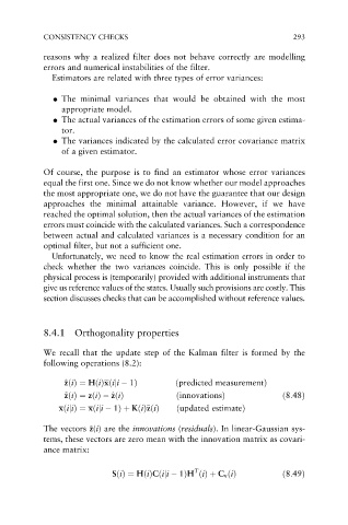
We recall that the update step of the Kalman filter is formed by the
following operations (8.2):
z
^ zðiÞ¼ HðiÞxðiji 1Þ ðpredicted measurementÞ
z
z
~ zðiÞ¼ zðiÞ ^ zðiÞ ðinnovationsÞ ð8:48Þ
z
xðiijÞ ¼ xðiji 1Þþ KðiÞ~ zðiÞ ðupdated estimateÞ
z
The vectors ~ z(i) are the innovations (residuals). In linear-Gaussian sys-
tems, these vectors are zero mean with the innovation matrix as covari-
ance matrix:

T
SðiÞ¼ HðiÞCðiji 1ÞH ðiÞþ C v ðiÞ ð8:49Þ