Page 32 - Complementarity and Variational Inequalities in Electronics

22 Complementarity and Variational Inequalities in Electronics

which is equivalent to the convex subdifferential relation

(i).
V ∈ ∂
R +
The electrical superpotential of the ideal diode is

(x).
ϕ D (x) =
R +
Then

∗
D
ϕ (z) =
R − (z).
We have also
⎧
⎪ R − if x = 0
⎪
⎨
∂ϕ D (x) = 0 if x> 0
⎪
⎪
∅ if x< 0
⎩
and
⎧
if z = 0
⎪ R +
⎪
⎨
∗
∂ϕ (z) = 0 if z< 0
D
⎪
⎪
∅ if z> 0.
⎩
The complementarity relation can thus be written as
∗
∗
V ∈ ∂ϕ D (i) ⇐⇒ i ∈ ∂ϕ (V ) ⇐⇒ ϕ D (i) + ϕ (V ) = iV.
D
D
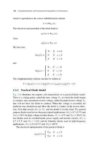
2.3.2 Practical Diode Model
Fig. 2.14 illustrates the ampere–volt characteristic of a practical diode model.
There is a voltage point, called the knee voltage V 1 , at which the diode begins
to conduct, and a maximum reverse voltage, called the peak reverse voltage V 2 ,
that will not force the diode to conduct. When this voltage is exceeded, the
depletion may breakdown and allow the diode to conduct in the reverse direc-
tion. Note that usually |V 2 | |V 1 | and the model is locally ideal. For general
purpose diodes used in low-frequency/speed applications, |V 1 | 0.7–2.5 V and
|V 2 | 5 kV; for high-voltage rectifier diodes, |V 1 | 10 V and |V 2 | 30 kV; for
fast diodes used in switched-mode power supply and inverter circuits, |V 1 |
0.7–1.5 V and |V 2 | 3 kV; and for Schottky diodes used in high-frequency
applications, |V 1 | 0.2–0.9 V and |V 2 | 100 V.
The electrical superpotential of the practical diode is

V 1 x if x ≥ 0
ϕ PD (x) =
V 2 x if x< 0.