Page 28 - Complementarity and Variational Inequalities in Electronics

18 Complementarity and Variational Inequalities in Electronics

o
∗
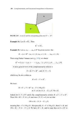
FIGURE 2.10 A cone K and the corresponding polar cone K =−K .
n
Example 14. Let K = R . Then
+
n
∗
K = R .
+
n
Example 15. Let a 1 ,a 2 ,...,a m ∈ R be given vectors. Set
n
K ={x ∈ R :
a 1 ,x ≥ 0,
a 2 ,x ≥ 0,...,
a m ,x ≥ 0}.
Then using Farkas’ lemma (see e.g. [83]), we obtain

∗
K ={λ 1 a 1 + λ 2 a 2 + ··· + λ m a m : λ 1 ≥ 0,λ 2 ≥ 0,...,λ m ≥ 0}.
A more general form of the complementarity relation is

∗
U ∈ K,V ∈ K , and
U,V = 0,
which may be also written as

∗
K U ⊥ V ∈ K .
We have:
∗
K U ⊥ V ∈ K ⇔−V ∈ ∂
K (U)
⇔ V ∈ K &
V,h − U ≥ 0, ∀h ∈ K.
n
∗
Indeed, let U,V ∈ R satisfy the complementarity relation K U ⊥ V ∈ K .
Then (∀h ∈ K) :
V,h ≥ 0, and since
V,U = 0, we see that
(∀h ∈ K) :
V,h − U ≥ 0,

meaning that −V ∈ ∂
K (U). Reciprocally, if −V ∈ ∂
K (U), then U ∈ K and
(∀h ∈ K) :
V,h − U ≥ 0. We have 2U ∈ K, and we may thus set h = 2U to