Page 24 - Complementarity and Variational Inequalities in Electronics

14 Complementarity and Variational Inequalities in Electronics

∗
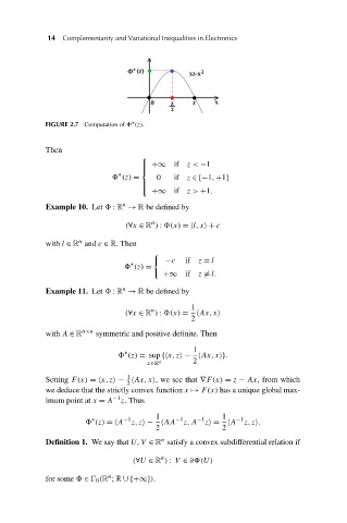
FIGURE 2.7 Computation of (z).

Then
⎧
⎪ +∞ if z< −1
⎪
⎨
∗
(z) = 0 if z ∈[−1,+1]
⎪
+∞ if z> +1.
⎪
⎩
n
Example 10. Let : R → R be defined by
n
(∀x ∈ R ) : (x) =
l,x + c
n
with l ∈ R and c ∈ R. Then

−c if z = l
∗
(z) =
+∞ if z = l.
n
Example 11. Let : R → R be defined by
1
n
(∀x ∈ R ) : (x) =
Ax,x
2
with A ∈ R n×n symmetric and positive definite. Then
1
∗
(z) = sup {
x,z −
Ax,x }.
x∈R n 2
1
Setting F(x) =
x,z −
Ax,x , we see that ∇F(x) = z − Ax, from which
2
we deduce that the strictly convex function x ð F(x) has a unique global max-
imum point at x = A −1 z. Thus
1 −1 −1 1 −1
−1
∗
(z) =
A z,z −
AA z,A z =
A z,z .
2 2
n
Definition 1. We say that U,V ∈ R satisfy a convex subdifferential relation if
n
(∀U ∈ R ) : V ∈ ∂ (U)
n
for some ∈ 0 (R ;R ∪{+∞}).