Page 26 - Complementarity and Variational Inequalities in Electronics

16 Complementarity and Variational Inequalities in Electronics

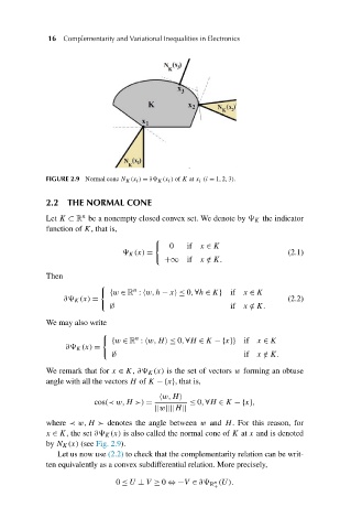
FIGURE 2.9 Normal cone N K (x i ) = ∂
K (x i ) of K at x i (i = 1,2,3).

2.2 THE NORMAL CONE

n
Let K ⊂ R be a nonempty closed convex set. We denote by
K the indicator
function of K, that is,

0 if x ∈ K

K (x) = (2.1)
+∞ if x/∈ K.
Then
n

{w ∈ R :
w,h − x 0,∀h ∈ K} if x ∈ K
∂
K (x) = (2.2)
∅ if x/∈ K.
We may also write

n
{w ∈ R :
w,H 0,∀H ∈ K −{x}} if x ∈ K
∂
K (x) =
∅ if x/∈ K.
We remark that for x ∈ K, ∂
K (x) is the set of vectors w forming an obtuse
angle with all the vectors H of K −{x}, that is,

w,H
cos(≺ w,H ) = ≤ 0,∀H ∈ K −{x},
||w||||H||
where ≺ w,H denotes the angle between w and H. For this reason, for
x ∈ K,the set ∂
K (x) is also called the normal cone of K at x and is denoted
by N K (x) (see Fig. 2.9).
Let us now use (2.2) to check that the complementarity relation can be writ-
ten equivalently as a convex subdifferential relation. More precisely,
0 ≤ U ⊥ V ≥ 0 ⇔−V ∈ ∂
R (U).
n
+