
Page 33 - Complementarity and Variational Inequalities in Electronics
P. 33
The Convex Subdifferential Relation Chapter | 2 23
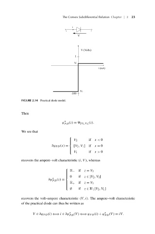
FIGURE 2.14 Practical diode model.
Then
ϕ ∗ (z) =
[V 2 ,V 1 ] (z).
PD
We see that
⎧
if x< 0
⎪ V 2
⎪
⎨
∂ϕ PD (x) = [V 2 ,V 1 ] if x = 0
⎪
⎪
⎩
V 1 if x> 0
recovers the ampere–volt characteristic (i,V ), whereas
⎧
⎪ R − if z = V 2
⎪
⎪
0 if z ∈]V 2 ,V 1 [
⎪
⎨
∗
∂ϕ PD (z) =
⎪ R +
⎪ if z = V 1
⎪
⎪
⎩
∅ if z ∈ R\[V 2 ,V 1 ]
recovers the volt–ampere characteristic (V,i). The ampere–volt characteristic
of the practical diode can thus be written as
V ∈ ∂ϕ PD (i) ⇐⇒ i ∈ ∂ϕ ∗ (V ) ⇐⇒ ϕ PD (i) + ϕ ∗ (V ) = iV.
PD PD