Page 58 - Complementarity and Variational Inequalities in Electronics

A Variational Inequality Theory Chapter | 4 49

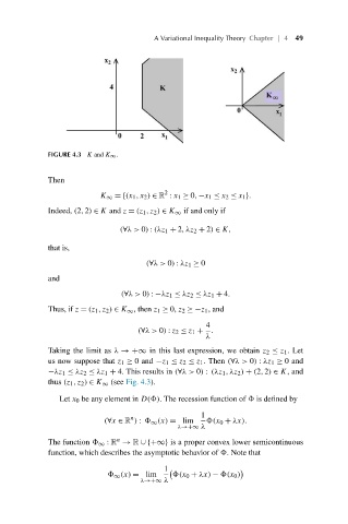
FIGURE 4.3 K and K ∞ .

Then
2
K ∞ ={(x 1 ,x 2 ) ∈ R : x 1 ≥ 0,−x 1 ≤ x 2 ≤ x 1 }.
Indeed, (2,2) ∈ K and z = (z 1 ,z 2 ) ∈ K ∞ if and only if

(∀λ> 0) : (λz 1 + 2,λz 2 + 2) ∈ K,

that is,
(∀λ> 0) : λz 1 ≥ 0
and

(∀λ> 0) :−λz 1 ≤ λz 2 ≤ λz 1 + 4.
Thus, if z = (z 1 ,z 2 ) ∈ K ∞ , then z 1 ≥ 0, z 2 ≥−z 1 , and

4
(∀λ> 0) : z 2 ≤ z 1 + .
λ
Taking the limit as λ →+∞ in this last expression, we obtain z 2 ≤ z 1 .Let
us now suppose that z 1 ≥ 0 and −z 1 ≤ z 2 ≤ z 1 . Then (∀λ> 0) : λz 1 ≥ 0 and
−λz 1 ≤ λz 2 ≤ λz 1 + 4. This results in (∀λ> 0) : (λz 1 ,λz 2 ) + (2,2) ∈ K, and
thus (z 1 ,z 2 ) ∈ K ∞ (see Fig. 4.3).

Let x 0 be any element in D( ). The recession function of is defined by
1
n
(∀x ∈ R ) : ∞ (x) = lim (x 0 + λx).
λ→+∞ λ
n
The function ∞ : R → R ∪{+∞} is a proper convex lower semicontinuous
function, which describes the asymptotic behavior of . Note that

1
∞ (x) = lim (x 0 + λx) − (x 0 )
λ→+∞ λ