Page 66 - Complementarity and Variational Inequalities in Electronics

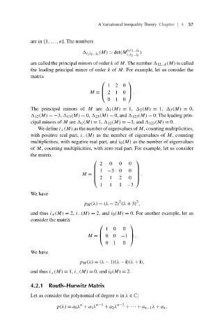
A Variational Inequality Theory Chapter | 4 57

are in {1,...,n}. The numbers

(M) = det(M i 1 i 2 ...i k )
i 1 i 2 ...i k
i 1 i 2 ...i k
are called the principal minors of order k of M. The number 12...k (M) is called
the leading principal minor of order k of M. For example, let us consider the
matrix
⎛ ⎞
1 2 0
⎟
M = ⎝ 2 1 0 ⎠ .
⎜
0 1 0
The principal minors of M are 1 (M) = 1, 2 (M) = 1, 3 (M) = 0,
12 (M) =−3, 13 (M) = 0, 23 (M) = 0, and 123 (M) = 0. The leading prin-
cipal minors of M are 1 (M) = 1, 12 (M) =−3, and 123 (M) = 0.
We define i + (M) as the number of eigenvalues of M, counting multiplicities,
with positive real part, i − (M) as the number of eigenvalues of M, counting
multiplicities, with negative real part, and i 0 (M) as the number of eigenvalues
of M, counting multiplicities, with zero real part. For example, let us consider
the matrix
⎛ ⎞
2 0 0 0
⎜ 1 −30 ⎟
⎜
⎟.
0 ⎟
⎝ 2 1 2 0 ⎠
M = ⎜
1 1 1 −3
We have
2
2
p M (λ) = (λ − 2) (λ + 3) ,
and thus i + (M) = 2, i − (M) = 2, and i 0 (M) = 0. For another example, let us
consider the matrix
⎛ ⎞
1 0 0
M = ⎝ 0 0 −1 ⎠ .
⎟
⎜
0 1 0
We have

p M (λ) = (λ − 1)(λ − i)(λ + i),
and thus i + (M) = 1, i − (M) = 0, and i 0 (M) = 2.

4.2.1 Routh–Hurwitz Matrix

Let us consider the polynomial of degree n in λ ∈ C:
n
p(λ) = a 0 λ + a 1 λ n−1 + a 2 λ n−2 + ··· + a n−1 λ + a n ,