Page 146 - Computational Colour Science Using MATLAB

IMPLEMENTATIONS AND EXAMPLES 133

plot(ref,py,’ko’);
hold on
plot([0 1], [0 1], ’k-’);
axis([0 1 0 1])
disp(255*py’)

subplot(3,2,5)
plot(b,ref,’ko’);
x = linspace(0,1,11);
y = polyval(pb1,x);
hold on
plot(x,y,’k-’);
ylabel(’Y’)
xlabel(’B channel’);
axis([0 1 0 1])
subplot(3,2,6)
py = polyval(pb1,b);
plot(ref,py,’bo’);
hold on
plot([0 1], [0 1], ’k-’);
axis([0 1 0 1])
disp(255*py’)

end

out = [pr1; pg1; pb1];

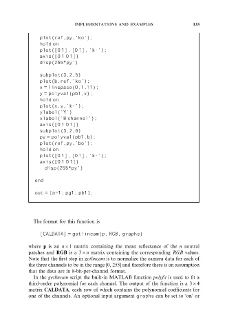
The format for this function is

[CALDATA] = getlincam(p, RGB, graphs)

where p is an n61 matrix containing the mean reflectance of the n neutral
patches and RGB is a 36n matrix containing the corresponding RGB values.
Note that the first step in getlincam is to normalize the camera data for each of
the three channels to be in the range [0, 255] and therefore there is an assumption
that the data are in 8-bit-per-channel format.
In the getlincam script the built-in MATLAB function polyfit is used to fit a
third-order polynomial for each channel. The output of the function is a 364
matrix CALDATA, each row of which contains the polynomial coefficients for
one of the channels. An optional input argument graphs can be set to ‘on’ or