Page 147 - Computational Colour Science Using MATLAB

134 CHARACTERIZATION OF CAMERAS

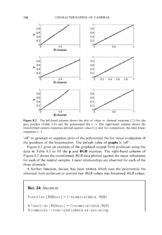
Figure 8.2 The left-hand column shows the plot of value vs. channel response (*) for the
grey patches (Table 8.1) and the polynomial fits (– ). The right-hand column shows the
transformed camera responses plotted against value (*) and, for comparison, the ideal linear
responses (– )
‘off’ to generate or suppress plots of the polynomial fits for visual evaluation of
the goodness of the linearization. The default value of graphs is ‘off’.
Figure 8.2 gives an example of the graphical output from getlincam using the
data in Table 8.1 to fill the p and RGB matrices. The right-hand column of
Figure 8.2 shows the transformed RGB data plotted against the mean reflectance
for each of the neutral samples. Linear relationships are observed for each of the
three channels.
A further function, lincam, has been written which uses the polynomial fits
obtained from getlincam to convert raw RGB values into linearized RGB values.

Box 24: lincam.m

function [RGBout] = lincam(caldata, RGB)

% function [RGBout] = lincam(caldata,RGB)
% computes linearized camera values using