Page 150 - Computational Colour Science Using MATLAB

IMPLEMENTATIONS AND EXAMPLES 137
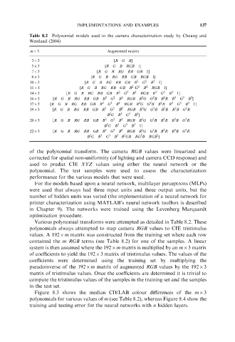
Table 8.2 Polynomial models used in the camera characterization study by Cheung and
Westland (2004)
m63 Augmented matrix

363 [RGB]
563 [RGBRGB 1]
763 [RG B RG RBGB 1]
863 [R G B RG RB GB RGB 1]
1063 [R G B RG RB GB R 2 G 2 B 2 1]
2
1163 [RG BRGRBGBR G 2 B 2 RGB 1]
1463 [RG BRGRBGBR 2 G 2 B 2 RGB R 3 G 3 B 3 1]
2
2
3
2
1663 [RG B RG RBGB R 2 G 2 B 2 RGB R GG BB RR 3 G 3 B ]
2
2
2
1763 [R G B RG RB GB R 2 G 2 B 2 RGB R GG BB RR 3 G 3 B 3 1]
2
2
2
2
2
1963 [R G B RG RB GB R 2 G 2 B 2 RGB R GG BB RR BG R
2
3
B GR 3 G 3 B ]
2
2
2
2
2
2063 [R G B RG RB GB R 2 G 2 B 2 RGB R GG BB RR BG R
2
B GR 3 G 3 B 3 1]
2
2
2
2
2
2263 [R G B RG RB GB R 2 G 2 B 2 RGB R GG BB RR BG R
2
2
2
2
B GR 3 G 3 B 3 R GB RG B RGB ]
of the polynomial transform. The camera RGB values were linearized and
corrected for spatial non-uniformity (of lighting and camera CCD response) and
used to predict CIE XYZ values using either the neural network or the
polynomial. The test samples were used to assess the characterization
performance for the various models that were used.
For the models based upon a neural network, multilayer perceptrons (MLPs)
were used that always had three input units and three output units, but the
number of hidden units was varied (the implementation of a neural network for
printer characterization using MATLAB’s neural network toolbox is described
in Chapter 9). The networks were trained using the Levenberg–Marquardt
optimization procedure.
Various polynomial transforms were attempted as detailed in Table 8.2. These
polynomials always attempted to map camera RGB values to CIE tristimulus
values. A 1926m matrix was constructed from the training set where each row
contained the m RGB terms (see Table 8.2) for one of the samples. A linear
system is then assumed where the 1926m matrix is multiplied by an m63 matrix
of coefficients to yield the 19263 matrix of tristimulus values. The values of the
coefficients were determined using the training set by multiplying the
pseudoinverse of the 1926m matrix of augmented RGB values by the 19263
matrix of tristimulus values. Once the coefficients are determined it is trivial to
compute the tristimulus values of the samples in the training set and the samples
in the test set.
Figure 8.3 shows the median CIELAB colour differences of the m63
polynomials for various values of m (see Table 8.2), whereas Figure 8.4 show the
training and testing error for the neural networks with n hidden layers.