Page 179 - Computational Colour Science Using MATLAB

166 MULTISPECTRAL IMAGING
where a is the weight of the jth basis function for the ith sample. The basis
i,j
functions are themselves functions of wavelength but are not constrained to be
between the range [0,1] nor even to be positive at all wavelengths. The number of
basis functions n usually is quite small and the weights for each reflectance
spectrum define a projection of the reflectance spectrum onto the n-dimensional
space of the basis functions. Such linear models of reflectance spectra and
illuminant power distributions are useful because they provide an efficient
method for representing and storing P and E. The linear models are also useful
because they lead to simple estimation algorithms for P and E given the three
sensor responses r (r could be the responses of the cones in the human visual
system or the responses of a trichromatic imaging system).
We can therefore rewrite Equation (10.4) as

r ¼ MBa, ð10.6Þ

where the columns of the 3163 matrix B hold the first three basis functions of a
linear model of reflectance spectra and the 361 matrix a holds the weights that
define the particular spectrum that we are trying to recover (note that p ¼ Ba). If
we group together the term MB (multiplying a 3631 matrix by a 3163 matrix),
then we can see that this is a 363 matrix whose entries are all known. The only
unknown is a, the weights. We can therefore rearrange Equation (10.6) to
produce
1
a ¼ðMBÞ r, ð10.7Þ

which allows a to be computed by standard procedures. Once a has been
determined the reflectance spectrum can be recovered using p ¼ Ba. This analysis
illustrates two aspects of the role of linear models. First, linear models represent
a priori knowledge about the likely set of inputs. Linear models may be used to
allow spectral information to be recovered from three sensor responses.
Secondly, linear models work smoothly with the imaging equations. Since the
imaging equations are linear, the estimation methods remain linear and simple.
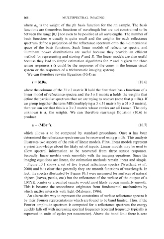
Figure 10.1 shows a set of five typical reflectance spectra (Westland et al.,
2000) and it is clear that generally they are smooth functions of wavelength. In
fact, the spectra illustrated by Figure 10.1 were measured for surfaces of natural
objects (leaves, petals, etc.) but the reflectance of the surface of the output of a
CMYK printer or a painted sample would most likely appear similarly smooth.
This is because the smoothness originates from fundamental mechanisms by
which matter interacts with light (Maloney, 1986).
An alternative way to represent the constraints of surface reflectance spectra is
by their Fourier representations which are found to be band limited. Thus, if the
Fourier amplitude spectrum is computed for a reflectance spectrum the energy
quickly falls off with increasing spectral frequency (spectral frequency typically is
expressed in units of cycles per nanometer). Above the band limit there is zero